WIXLIB

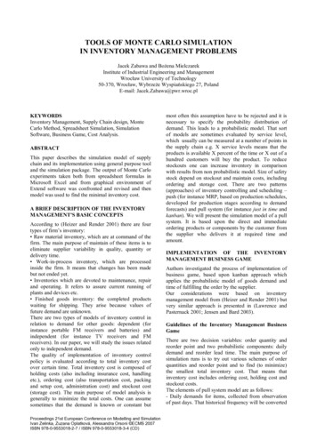
TOOLS OF MONTE CARLO SIMULATIONIN INVENTORY MANAGEMENT PROBLEMSJacek Zabawa and Bożena MielczarekInstitute of Industrial Engineering and ManagementWrocław University of Technology50-370, Wrocław, Wybrzeże Wyspiańskiego 27, PolandE-mail: Jacek.Zabawa@pwr.wroc.plKEYWORDSInventory Management, Supply Chain design, MonteCarlo Method, Spreadsheet Simulation, SimulationSoftware, Business Game, Cost Analysis.ABSTRACTThis paper describes the simulation model of supplychain and its implementation using general purpose tooland the simulation package. The output of Monte Carloexperiments taken both from spreadsheet formulas inMicrosoft Excel and from graphical environment ofExtend software was confronted and revised and thenmodel was used to find the minimal inventory cost.A BRIEF DESCRIPTION OF THE INVENTORYMANAGEMENT'S BASIC CONCEPTSAccording to (Heizer and Render 2001) there are fourtypes of firm’s inventory: Raw material inventory, which are at command of thefirm. The main purpose of maintain of these items is toeliminate supplier variability in quality, quantity ordelivery time. Work-in-process inventory, which are processedinside the firm. It means that changes has been madebut not ended yet. Inventories which are devoted to maintenance, repairand operating. It refers to assure current running ofplants and devices etc. Finished goods inventory: the completed productswaiting for shipping. They arise because values offuture demand are unknown.There are two types of models of inventory control inrelation to demand for other goods: dependent (forinstance portable FM receivers and batteries) andindependent (for instance TV receivers and FMreceivers). In our paper, we will study the issues relatedonly to independent demand.The quality of implementation of inventory controlpolicy is evaluated according to total inventory costover certain time. Total inventory cost is composed ofholding costs (also including insurance cost, handlingetc.), ordering cost (also transportation cost, packingand setup cost, administration cost) and stockout cost(storage cost). The main purpose of model analysis isgenerally to minimize the total costs. One can assumesometimes that the demand is known or constant butProceedings 21st European Conference on Modelling and SimulationIvan Zelinka, Zuzana Oplatková, Alessandra Orsoni ECMS 2007ISBN 978-0-9553018-2-7 / ISBN 978-0-9553018-3-4 (CD)most often this assumption have to be rejected and it isnecessary to specify the probability distribution ofdemand. This leads to a probabilistic model. That sortof models are sometimes evaluated by service level,which usually can be measured at a number of points inthe supply chain e.g. X service levels means that theproducts is available X percent of the time or X out of ahundred customers will buy the product. To reducestockouts one can increase inventory in comparisonwith results from non probabilistic model. Size of safetystock depend on stockout and maintain costs, includingordering and storage cost. There are two patterns(approaches) of inventory controlling and scheduling –push (for instance MRP, based on production schedules,developed for production stages according to demandforecasts) and pull system (for instance just in time andkanban). We will present the simulation model of a pullsystem. It is based upon the direct and immediateordering products or components by the customer fromthe supplier who delivers it at required time andamount.IMPLEMENTATION OF THE INVENTORYMANAGEMENT BUSINESS GAMEAuthors investigated the process of implementation ofbusiness game, based upon kanban approach whichapplies the probabilistic model of goods demand andtime of fulfilling the order by the supplier.Our considerations were based on inventorymanagement model from (Heizer and Render 2001) butvery similar approach is presented in (Lawrence andPasternack 2001; Jensen and Bard 2003).Guidelines of the Inventory Management BusinessGameThere are two decision variables: order quantity andreorder point and two probabilistic components: dailydemand and reorder lead time. The main purpose ofsimulation runs is to try out various schemes of orderquantities and reorder point and to find (to minimize)the smallest total inventory cost. That means thatinventory cost includes ordering cost, holding cost andstockout costs.The elements of pull system model are as follows:- Daily demands for items, collected from observationof past days. That historical frequency will be converted

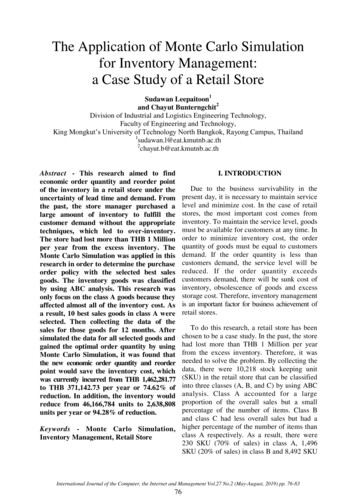
into a probability distribution and cumulativedistribution for the variable daily demand- Lead time (in days), collected from observations ofpast orders. That historical frequency will be convertedinto a probability distribution and cumulativedistribution for the variable lead time- Beginning inventory (in units)- Reorder point (in units)- Order quantity (in units)- Cost of placing order- Holding cost per unit- Cost of each lost sale (stockout).Apart from the above mentioned, the additionalassumptions were formulated:- Orders (if necessary) are placed at the end of the day:the day’s ending inventory is checked and if inventoryis less or equal reorder point then order is placed.- Lead time equal 1 day stands for that the order willarrive next morning after next day.- After arriving at the morning, order quantity is addedto inventory, before receiving of the new demand.our spreadsheet and the results discussed in (Heizer andRender 2001) are statistically similar. For example,during applying ANOVA test we obtained critical valueof the F distribution (significance level 0.05, 1 and 58degrees of freedom) equal 4 and source has F-valueequal 1.55 and that means that both populations are notvaried.Implementation of Monte Carlo Simulation in aSpreadsheetStages of spreadsheet’s simulation building wereformulated for instance at (Seila 2002). According todefinition of Monte Carlo simulation (Lawrence andPasternack 2001), simulated events take place randomlyand match the description of the theoretical probabilitiesderived from acquired experiences. The process offundamental importance in Monte Carlo simulation iscalled random number mapping and consists inmatching the random number with simulated events(when they occur and how long they last). Manyexamples of applications of Monte Carlo method withMicrosoft Excel spreadsheet as a base for makingsimulation experiments can be found. See (Heizer andRender 2001), (Jensen and Bard 2003) and (Lawrenceand Pasternack 2001). We did similar task, but usingmore flexible formulas and data tables (see screenshotsat Figures (1, 2 and 3) for collecting simulationoutcomes. Figure (1) presents the frequencies ofdemand and lead time, probabilities and cumulativeprobabilities and the way of assigning random-numberintervals to get the proper outcomes in a computersimulation. Figure (2) shows one of 20-day simulationruns. Average and total number of units received,simulated demand, ending inventory, stockouts andplaced orders are calculated. Figure (3) presents datatable with one variable, used to collect 60 replications(runs) of simulated total stockouts during 20 days. Ashort procedure in Visual Basic is necessary to collectoutput values and to ensure correct calculation aftersheet refreshing. Other (missing) values of problemdescription parameter, like reorder point, quantity orderand beginning inventory are visible in Figures (1 and 2).We will use the data also to validate Monte Carloapproach model in Extend, Imagine That Inc.environment. It's worth mentioning, that outcomes ofFigures 1: First Part of our MS Excel SpreadsheetThe key formulas of our spreadsheet are as follows(starting from the cells in 4th row, from column B):Number of units received: “ IF(L3 A4; B 32;0)”.Beginning inventory: “ F3 B4”.Simulated demand: “ INDEX( B 35 B 41MATCH(D4; G 35: G 41;1))”First random number: “ E 31-INT(RAND()* E 31)”Ending inventory: “ IF(C4-E4 0;C4-E4;0)”Stockouts: “ IF(C4-E4 0;0;E4-C4)”Inventory not below reorder point?“ IF(F4 B 31;1;0)”Placing order: “ IF(AND(H4 1;A4 L3);1;0)”Second random number:

“ IF(AND(H4 1;A4 L3); E 32INT(RAND()* E 32);0)”Planned arriving day: IF(IF( K4 0; A4 K4 1; L3) A4;IF( K4 0; A4 K4 1; L3);0)Fourth row of Figure (3) in columns O, Q, S containsformula “ B26” and other rows in column O, Q, Scontain formula “ TABLE(;P2)”.RUNNING MONTEMODEL IN EXTENDCARLOSIMULATIONSIntroduction to Modeling with Extend softwareFigures 2: Second Part of Our MS Excel SpreadsheetThe equivalent model was built in graphicalenvironment of Extend software. Then, two modelswere compared and validated by confronting theoutcomes. Modelling in Extend (Krahl 2002) consists inusing pre-built modelling components to build andanalyse system. This approach is also applied in othersoftware like Arena, Flexim and others. As we see onFigure (4), results from this model implementation issimilar (average 15.467 and standard deviation 5.95) toMS Excel spreadsheet outcomes, Figure (3). It is worthmentioning that it was necessary to make twocorrections into object’s way in model. First, we have tosecure to the arriving „demand” object a very smallamount of time after the arriving of „order” object (it isbeginning of the day), second – we have to add 1 dayfor all lead times shown in Figure (1) before placingthis information in Input Random Number (the blockwith histogram icon). After introductory validation ofour Extend model, we think that discrete event modelbuilt in Extend is more flexible, because it is possible toeasily prolong simulated time and the number ofreplications (runs), to see the animation of objectsduring the run and to optimise model variables(minimization of total cost). We will try to prove it inthe next section.Guidelines of the Inventory Management BusinessGame with Cost AccountingFigures 3: Tabularization of Simulation Outcomes of 60Runs.Simulated lead time:“ IF(L3 A4 1;IF(I4 1;INDEX(B47:B50;MATCH(J4;sG47:G50;1));0);0)”We prepared the equivalent model to the previous oneusing the Extend software, but we extended it by costcoefficient taken from the example of inventory systemsimulation given in (Jensen and Bard 2003). Next, wevalidated it by comparing the optimal values found inour simulations with these presented in the book.The set of assumptions are as follows: the dailydemand oscillates between 6 and 16 units, lead timeoscillates between 1 and 5 day, initial inventory is 50units, cost per day of unit holding is 10 cents, cost oflost sale (stockout) is 5, ordering cost is 20, reorderpoint is 35 and order quantity is 70 units. Note: in thissituation, lead time equal to 1 day means that the orderwill arrive next morning.

Figures 4: Monte Carlo Method in Inventory Management Model Built in Extend Software.Equivalent of a Spreadsheet Simulation Model

Figures 5: Inventory Management Model with Cost Calculations, Ready for Optimisation.