Transcription
An Asymptote tutorialCharles Staats IIIFebruary 15, 2021Contents1 First Steps1.1 Introduction . . . . . . . . . . . . . . . . . . . . . . . . . . . . . .1.2 Hello World . . . . . . . . . . . . . . . . . . . . . . . . . . . . . .1.3 Interpreting the documentation . . . . . . . . . . . . . . . . . . .2 Drawing a two-dimensional image2.1 Lines and sizing . . . . . . . . . . . . . . . . . . .2.2 Arrowheads . . . . . . . . . . . . . . . . . . . . .2.3 Curved paths . . . . . . . . . . . . . . . . . . . .2.4 Markers on paths . . . . . . . . . . . . . . . . . .2.5 Circles and ellipses . . . . . . . . . . . . . . . . .2.6 Boxes and polygons . . . . . . . . . . . . . . . .2.7 Transformations: shifting, scaling, rotating, etc. .2.8 Arcs and margins . . . . . . . . . . . . . . . . . .2.9 Filling a region . . . . . . . . . . . . . . . . . . .2.10 Drawing a dot at a point . . . . . . . . . . . . . .2.11 Named paths and variables . . . . . . . . . . . .2.12 Clipping a picture . . . . . . . . . . . . . . . . .2.13 Path times and subpaths . . . . . . . . . . . . . .2.14 The Law of Janet . . . . . . . . . . . . . . . . . .2.15 Intersections and arrays and subpaths . . . . . .2.16 Tangent lines . . . . . . . . . . . . . . . . . . . .2.17 Drawing disconnected paths . . . . . . . . . . . .2.18 Graphing functions . . . . . . . . . . . . . . . . .2.19 Parametric graphs . . . . . . . . . . . . . . . . .2.20 Implicitly defined curves; building arrays . . . . .2.21 The filldraw command . . . . . . . . . . . . . . .2.22 Adding text . . . . . . . . . . . . . . . . . . . . .2.23 Adding multiple labels to a single path . . . . . .2.24 Drawing objects of a fixed (unscalable) size . . .2.25 Drawing objects shifted by an unscalable amount2.26 The two-dimensional picture: final result . . . . 8404448
3 Three-dimensional images3.1 Hello Sphere . . . . . . . . . . . . . . . . . . .3.2 Drawing lines in 3d . . . . . . . . . . . . . . .3.3 Vector graphics in 3d . . . . . . . . . . . . . .3.4 High-resolution rasterized images . . . . . . .3.5 Three-dimensional paths . . . . . . . . . . . .3.5.1 Parallelograms and 3d boxes . . . . .3.5.2 Circles and arcs . . . . . . . . . . . . .3.5.3 Planar curves . . . . . . . . . . . . . .3.5.4 Parametric curves . . . . . . . . . . .3.6 Surfaces of revolution . . . . . . . . . . . . .3.6.1 optional parameters . . . . . . . . . .3.7 Points of view; projections . . . . . . . . . . .3.7.1 Oblique projection . . . . . . . . . . .3.7.2 Perspective . . . . . . . . . . . . . . .3.7.3 Orthographic projection . . . . . . . .3.7.4 General recommendation . . . . . . .3.8 Predefined solids . . . . . . . . . . . . . . . .3.9 Three-dimensional transforms . . . . . . . . .3.10 Simple planar surfaces . . . . . . . . . . . . .3.11 Lighting . . . . . . . . . . . . . . . . . . . . .3.12 Planar surfaces with holes . . . . . . . . . . .3.13 Arrowheads in three dimensions . . . . . . . .3.13.1 Fancy 3d arrowheads . . . . . . . . . .3.13.2 Plain arrowheads in 3d . . . . . . . . .3.13.3 3d arrows in interactive mode . . . . .3.14 Labels in three dimensions . . . . . . . . . . .3.15 Layering: moving objects closer to the camera3.16 Complex scaling with unitsize() . . . . . .3.17 Writing on surfaces . . . . . . . . . . . . . . .3.18 Subtleties in drawing surfaces . . . . . . . . .3.18.1 Shading, lighting, and material . . . .3.18.2 Transparency . . . . . . . . . . . . . .3.18.3 Gridlines . . . . . . . . . . . . . . . .4 Building surfaces4.1 Predefined solids . . . . . . . . . . . . . . .4.2 Cylinders and cones over an arbitrary base4.3 Surfaces of revolution . . . . . . . . . . . .4.4 Parametric surfaces . . . . . . . . . . . . . .4.5 Graphs of functions of two variables . . . .4.6 Implicitly defined surfaces . . . . . . . . . .4.6.1 The smoothcontour3 module . . . .4.6.2 The contour3 module . . . . . . . .4.7 Cropping surfaces . . . . . . . . . . . . . . .92. 92. 92. 93. 93. 96. 97. 97. 99. 08082858586888989899292
ydxy f (x)f (x)xxDimensions of infinitesimally thinsheet:Area: πr2 π[f (x)]2Thickness: dxVolume: dV Area · thickness π[f (x)]2 dxA The complete code100B Installing Asymptote10511.1First StepsIntroductionJanet is a calculus teacher. She is currently teaching her students how to findvolumes of solids of revolution via the “disk method.” She would like to producea diagram to illustrate the method—something like the diagram shown on page 3.As an experienced user of TikZ, Janet does not think she would have troubleproducing the diagram in the top left of the figure. She also believes she could3
get the diagram in the bottom left with some fiddling. However, she simplydoes not believe the three-dimensional capabilities of TikZ are up to drawinga diagram like that in the top right—at least, not without far more time andfiddling than Janet is willing to put in for a single diagram.Janet’s husband Vincent is a programmer. He has some familiarity with theprogramming language Asymptote, which is especially designed to produce vectorgraphics and has some fairly substantial three-dimensional capabilities. Workingwith her husband, Janet decides to try to draw the figure using Asymptote.1.2Hello WorldJanet already has an up-to-date installation of TeXLive. On the off-chancethat this includes an Asymptote installation, she attempts a simple Hello Worldprogram. She uses her favorite text editor1 to produce a document consisting ofthe single linelabel("Hello world!");and saves it as hello world.asy. She then goes to the command line and typesasy hello world. The result is an eps file named hello world.eps. Openingit, she sees a single page with the following printed on it:2Hello world!Thus, to the surprise of both Janet and her husband, it appears that Asymptoteis already installed on her computer.3Since Janet uses pdflatex, she finds it annoying to import eps files, andwould prefer that the “graphic” be output in another format. Adding one lineto her Asymptote file causes it to output a pdf file instead:settings.outformat "pdf";label("Hello world!");Vincent notes that every line should end with a semicolon. Since TikZ behavesthe same way, Janet does not find this too difficult to remember.Now that Janet has a pdf file containing her “graphic,” she decides to importit into a latex file. Having done so, she is pleased to notice that Hello Worldis printed in the same font as the rest of her document (Computer Modern).However, she considers it unfortunate that the font size in the “graphic” is largerthan in the rest of her document. Vincent asks her what size she would like1 Sheis inclined to use TeXShop, since she already has it, but Aquamacs would reallybe more suitable. Vincent, who is a die-hard fan of the command line, recommends usingthe command-line editor nano. On a Windows machine, the simplest thing to use would beNotepad.2 Not including the yellow background, of course.3 This was more or less my experience, working on Mac OS X. If you are not fortunate enoughto have had this miracle happen to you, see Appendix B and the installation instructions inthe Asymptote manual.4
the font in her Asymptote graphics. Being told that the desired font size is 10points, he proposes the following:settings.outformat "pdf";defaultpen(fontsize(10pt));label("Hello world!");The result isHello world!which looks nicer with the rest of the document.1.3Interpreting the documentationThe label() command used in the Asymptote code above is described in Section4.4 of the Asymptote manual, with the following declaration:void label(picture pic currentpicture, Label L, pair position,align align NoAlign, pen p currentpen,filltype filltype NoFill)Janet finds this a bit overwhelming. Vincent suggests that she ignore everythingwith an sign in it, since those are all optional arguments, and think of such adeclaration simply aslabel(Label L, pair position);Essentially, if Janet wants to use this command to add a label to her picture,she should tell what Label to add and where to add it. For instance, the linelabel("Hello world", (0,0));would add the text “Hello world” to the picture at position (0, 0). Given thisdescription, Janet wonders why the program she already wrote worked; shouldn’tshe have been required to specify a position? Vincent confirms that accordingto the documentation, the line label("Hello world"); without any positionshould not have worked. He admits that the documentation is sometimes notcompletely accurate, which Janet does not find encouraging.It seems rather peculiar to Janet that the equals sign should be what indicatesthat an argument can be ignored. Vincent explains that the equals sign providesa default value; when there is a default value, the program knows what to do ifthe user does not specify a value.Here are the optional arguments for the label command:typenamedefault ntpictureNoAligncurrentpenNoFill5
These optional arguments behave something like key-value assignments. Forinstance, if Janet had wanted to change the text size of just the single line, ratherthan the entire picture, she could have set the key p to value fontsize(10pt)as follows:settings.outformat "pdf";label("Hello world", p fontsize(10pt));Note that fontsize(10pt) is an object of type pen, just as "Hello world"(including the quotation marks) is an object of type Label.4 The output is thesame as before, since the picture has only one piece of text:Hello worldJanet asks how to define a single key that can set several others, as in TikZstyles. Vincent says that this is not possible in Asymptote, although he can seehow it might be useful.22.1Drawing a two-dimensional imageLines and sizingHaving determined that Asymptote is already installed on her computer, Janetdecides to use it to draw a picture of the two-dimensional region that will berevolved. She could do this using TikZ, but Vincent recommends that she getsome basic practice drawing with Asymptote before tackling a three-dimensionalpicture. Here is, roughly, what Janet would like:4 Technically, "Hello world" is of type string, but strings can be treated as Labels inAsymptote.6
ydxy f (x)f (x)xxFirst of all, she tries drawing the x-axis as a line from ( 0.1, 0) to (2, 0), andthe y-axis as a line from (0, .1) to (0, 2);settings.outformat "pdf";draw((-.1,0) -- (2,0));draw((0,-.1) -- (0,2));The result is a mark that is barely visible because it is so short. Vincent letsJanet know this is because, by default, Asymptote interprets one unit to meanone point—roughly 0.035 centimeters. Janet thinks that the TikZ default of 1centimeter is much more reasonable. This can be arranged by adding the lineunitsize(1cm); to the code:settings.outformat "pdf";unitsize(1cm);draw((-.1,0) -- (2,0));draw((0,-.1) -- (0,2));The final product should be larger still, but is kept this size for now to savespace.There’s one more kind of sizing option for Asymptote: the size command.In its simplest usage, this command takes a single length for an argument—in thecode below, 3cm—and makes the final picture as large as possible, keeping thesame height-to-width ratio, such that neither the width nor the height exceedsthe specified dimension (3 centimeters).7
settings.outformat "pdf";size(3cm);draw((-.1,0) -- (2,0));draw((0,-.1) -- (0,2));The size command has several important variations: size(real, real) takes two dimensions—a maximum width and a maximum height, in that order. Thus, for instance, code that begins with thecommand size(2cm, 3cm); will ordinarily produce a picture that is either2 centimeters wide (and 3 centimeters tall) or a picture that is 3 centimeters tall (and 2 centimeters wide). In either case, the height-to-widthratio is preserved. If either argument in size(real, real) is zero, it is ignored. Thus,for instance, a picture that includes the command size(4cm, 0); willordinarily be scaled so that the width is exactly 4 centimeters. The heightwill be the “natural” height for this scaling factor. The command size(real, real, keepAspect false); will scale thewidth and height independently so that the resulting picture has exactlythe specified width and height, but the height-to-width ratio is allowed tochange. Thus, for instance, if a circle is drawn on a picture that has thistype of size command, the circle is likely to end up looking like an ellipse.One of Janet’s frustrations with TikZ has been that it is difficult to produce apicture that has exactly the desired width (or height). She is gratified to learnthat this will be much easier with Asymptote.2.2ArrowheadsWith the axis lines drawn, Janet thinks that they should have arrows indicatingthe directions. Vincent agrees that the axes should have arrows. Janet’s studentsdo not care about arrows.Arrows can be added on the end of the line by using the optional parameterarrow in the draw command:settings.outformat "pdf";unitsize(1cm);draw((-.1,0) -- (2,0), arrow Arrow);draw((0,-.1) -- (0,2), arrow Arrow);Vincent thinks this looks fairly nice. Janet wants to imitate the TEX-stylearrowheads , as she is used to being done in TikZ. Looking in the Asymptotemanual, she and Vincent find the following styles for arrowheads:8
Asymptote codeappearancedraw((0,0)--(1,0),arrow Arrow());draw((0,0)--(1,0),arrow ArcArrow());draw((0,0)--(1,0),arrow Arrow(SimpleHead));draw((0,0)--(1,0),arrow ArcArrow(SimpleHead));draw((0,0)--(1,0),arrow Arrow(HookHead));draw((0,0)--(1,0),arrow ArcArrow(HookHead));draw((0,0)--(1,0),arrow Arrow(TeXHead));The last, the TeXHead style, is more what Janet has in mind:settings.outformat "pdf";unitsize(1cm);draw((-.1,0) -- (2,0), arrow Arrow(TeXHead));draw((0,-.1) -- (0,2), arrow Arrow(TeXHead));2.3Curved pathsNext, Janet would like to draw the parabola function, which is supposed to looksomething like the graph of y x. Here’sa first attempt, with a path through the three points (0, 0), (1, 1), and (2, 2):settings.outformat "pdf";unitsize(1cm);draw((-.1,0) -- (2,0),arrow Arrow(TeXHead));draw((0,-.1) -- (0,2), arrow Arrow(TeXHead));draw((0,0) -- (1,1) -- (2,sqrt(2)));This does not look very nice at all. Substituting . for the connector -- can atleast make the path look smooth:settings.outformat "pdf";unitsize(1cm);draw((-.1,0) -- (2,0),arrow Arrow(TeXHead));draw((0,-.1) -- (0,2), arrow Arrow(TeXHead));draw((0,0) . (1,1) . (2,sqrt(2)));9
While this is a significant improvement, Janet would also like to make the tangentat the origin vertical. This can also be specified:settings.outformat "pdf";unitsize(1cm);draw((-.1,0) -- (2,0),arrow Arrow(TeXHead));draw((0,-.1) -- (0,2), arrow Arrow(TeXHead));draw((0,0){up} . (1,1) .(2,sqrt(2)));This looks more or less like what Janet had in mind.Note that up is really just short for (0,1). If Janet wanted a direction otherthan up (or down, right, or left, which are similar), she could specify thetangent direction explicitly as an ordered pair. For instance, here is a roughapproximation of a sine curve:settings.outformat "pdf";unitsize(0.5cm);draw((0,0){(1,1)} . {right}(pi/2,1). {(1,-1)}(pi,0) .{right}(3*pi/2,-1). {(1,1)}(2*pi, 0));Without the tangent directions specified, Asymptote does a very nice job ofconnecting the dots to form a smooth curve, but it doesn’t really look like a sinecurve. The ends in particular are much too steep:settings.outformat "pdf";unitsize(0.5cm);draw((0,0) . (pi/2,1) . (pi,0). (3*pi/2,-1) . (2*pi, 0));Except at the first and last points, the tangent direction at a point can bespecified either before or after the point—or, if a corner is desired, at both:settings.outformat "pdf";unitsize(0.5cm);draw((0,2) . {(1,-3)}(2,0){(1,1/3)}. (4,2));10
2.4Markers on pathsIf Janet wants to see what the points on a path were actually specified, she canuse the marker option to the draw command:settings.outformat "pdf";unitsize(0.5cm);draw((0,0) . (pi/2,1) . (pi,0). (3*pi/2,-1) . (2*pi, 0),marker MarkFill[0]);Designing your own markers is not that difficult, but requires more knowledgethan is currently available. Here are the built-in markers:built-in optiondescriptionMark[0]open circleMarkFill[0]filled circleMark[1]open triangleMarkFill[1]filled triangleMark[2]open squareMarkFill[2]filled squareMark[3]open pentagonMarkFill[3]filled pentagonMark[4]MarkFill[4]2.5open triangle(upside down)filled triangle(upside down)Mark[5]x-markMark[6]asteriskCircles and ellipsesThe pathunitcircleis a unit circle. The functionpath circle(pair c, real r);11appearance
returns a circle centered at c with radius r. The functionpath ellipse(pair c, real a, real b);produces an ellipse centered at c with horizontal diameter 2a and verticaldiameter 2b.settings.outformat "pdf";size(3cm);draw(circle((0,1), 0.5), red);draw(circle((1,0), 1.5), blue);draw(ellipse((1,0), 1.5, 0.5));2.6Boxes and polygonsThe functionpath box(pair a, pair b);returns a cyclic path that is a rectangle of which a and b are opposite corners:settings.outformat "pdf";unitsize(1cm);draw(box((0,0), (2,1)));The functionpath polygon(int n);returns a cyclic path that is a regular polygon with n sides, all of whose cornerslie on the unit circle:settings.outformat n(5), blue);2.7Transformations: shifting, scaling, rotating, etc.Janet observes that the polygon function above seems to be quite limited. Whathappens if she wants to draw a polygon at a different position, or a differentsize? Or upside down? Obviously, she could simply construct the path directly,but she thinks that the polygon function ought to allow for more flexibility.12
After consulting the documentation, Vincent realizes that such flexibility isnot necessary: Janet can still change the path after it has been created, butbefore it is drawn, using the transform type. Here’s an example of using ashift transform to draw several polygons side by side:settings.outformat "pdf";size(5cm);for (int n 3; n 7; n) {draw(shift(2.2*n, 0) *polygon(n));}Note also the use of a for loop to repeat the same code multiple times.Warning: Since Vincent is an experienced programmer in C-like languages, his first instinct is to use n instead of n to increment n.Unfortunately, this does not work in Asymptote; the creators decided to omitit because the corresponding n-- notation would interfere with the use of thenotation p -- q to indicate a line segment.!Here is some code demonstrating a number of useful transforms:settings.outformat "pdf";size(3cm,0);path p box((0,0), (1,1));draw(p, black linewidth(2.0pt));draw(shift(1,2)*p, blue);draw(xscale(1.6)*p, green);draw(yscale(1.4)*p, orange);draw(scale(1.8)*p, red);draw(rotate(60)*p, purple); /*Rotate 60degrees*/Transforms can be composed with one another using the * operator. Forinstance, to halve the height of a path, rotate it by 45 , and translate it two tothe left (in that order), you can do the following:settings.outformat "pdf";size(3cm,0);path p unitcircle;draw(p, black);path q shift(-2,0) * rotate(45) *yscale(0.5) * p;draw(q, blue);13
2.8Arcs and marginsThe functionpath arc(pair c, real r, real angle1, real angle2);creates an arc centered at c with radius r from angle1 to angle2 specified indegrees:settings.outformat 2,1) -- arc((2,1), 2, 60, 80) -- cycle);The arc goes counterclockwise if angle1 angle2, clockwise otherwise:settings.outformat -1.2)--(0,1.2));/* An arc from 270 to 0 goes clockwise. */draw(arc((0,0), r 1, angle1 270, angle2 0),arrow Arrow(TeXHead));settings.outformat -1.2)--(0,1.2));/* An arc from -90 to 0 goescounterclockwise. The same effect could beachieved by drawing an arc from 270 to360. */draw(arc((0,0), r 1, angle1 -90, angle2 0),arrow Arrow(TeXHead));There is another useful function for drawing arcs:path arc(pair c, explicit pair z1, explicit pair z2,bool direction CCW);This function produces an arc centered at c, starting at the point z1 and endingon the line from c to z2. The direction is specified by either direction CW(clockwise) or the default direction CCW (counterclockwise). This function canbe quite convenient for specifying an arc from one line to another:14
settings.outformat "pdf";size(3cm,0);draw((3,0) -- (0,0) -- (3,4));draw(arc((0,0), (2,0), (3,4)),arrow Arrow(TeXHead), red);draw(arc((0,0), (2,0), (3,4), direction CW),arrow Arrow(TeXHead), blue);dot((0,0)); dot((2,0)); dot((3,4));While this looks good at first glance, Janet is distressed that upon magnification,the two arrow tips both cross into the black line rather than stopping at its edge.Here is the code to fix this using the optional parameter margin for the draw()command:settings.outformat "pdf";size(3cm,0);draw((3,0) -- (0,0) -- (3,4));real linewidth linewidth(currentpen);/* A path drawn with margin ArrowMargins willbe shortened at the end by 0.5 linewidthand at the beginning by the fulllinewidth. */margin ArrowMargins TrueMargin(linewidth, 0.5 linewidth);draw(arc((0,0), (2,0), (3,4)), arrow Arrow(TeXHead), red,margin ArrowMargins);draw(arc((0,0), (2,0), (3,4), direction CW),arrow Arrow(TeXHead), blue, margin ArrowMargins);The dots have been omitted to show the full effect, which will nevertheless bevisible only on close inspection (probably with high zoom).2.9Filling a regionNext, Janet would like to fill the region under the half-parabola. This may beaccomplished by creating a cyclic path and filling it with the fill command:settings.outformat "pdf";unitsize(1cm);draw((-.1,0) -- (2,0), arrow Arrow(TeXHead));draw((0,-.1) -- (0,2), arrow Arrow(TeXHead));draw((0,0){up} . (1,1) . (2,sqrt(2)));fill((0,0){up} . (1,1) . (2,sqrt(2))-- (2,0) -- cycle);15
Note the use of cycle to close the path. Also note that the . and -- operatorscan be combined to produce a path that is curved some places and straightothers. If . cycle were used instead of --cycle, the path would be closedsmoothly:settings.outformat "pdf";unitsize(1cm);draw((-.1,0) -- (2,0), arrow Arrow(TeXHead));draw((0,-.1) -- (0,2), arrow Arrow(TeXHead));draw((0,0){up} . (1,1) . (2,sqrt(2))-- (2,0) . cycle);Returning to the originally desired picture, Janet really wants it filled with agray color rather than black. This is not hard to achieve—she can just add anoption to the fill command specifying what color she wants used.fill((0,0){up} . (1,1) . (2,sqrt(2)) -- (2,0)-- cycle, mediumgray);Janet almost immediately notices a problem: the filled area is covering otherthings, including half the arrowhead on the x-axis. This can be fixed by puttingthe fill command earlier, so that the other things get drawn on top of the filledarea:settings.outformat "pdf";unitsize(1cm);fill((0,0){up} . (1,1) . (2,sqrt(2))-- (2,0) -- cycle, mediumgray);draw((-.1,0) -- (2,0), arrow Arrow(TeXHead));draw((0,-.1) -- (0,2), arrow Arrow(TeXHead));draw((0,0){up} . (1,1) . (2,sqrt(2)));Janet thinks that looks much better. Vincent agrees.2.10Drawing a dot at a pointOne thing Janet imagines the fill command might be useful for is if she wantsto draw a point—say, for a scatter plot:16
settings.outformat "pdf";size(5cm,5cm);draw((0,0) -- (50,0), arrow Arrow(TeXHead));draw((0,0) -- (0,10), arrow Arrow(TeXHead));real r ill(circle((42,9),r));Vincent believes there may be trouble here, however, in case the plot needs tobe rescaled. For data plots like this, the actual x and y scales are typically notin the same units, so there is no reason to keep the aspect ratio constant:settings.outformat "pdf";size(5cm,5cm, keepAspect false);draw((0,0) -- (50,0),arrow Arrow(TeXHead));draw((0,0) -- (0,10),arrow Arrow(TeXHead));real r ill(circle((42,9),r));Unfortunately, this highlights a key weakness of drawing points by filling circles:the “points” obtained thus can change size and even shape when the picture isrescaled.Fortunately, there is a command designed for precisely this sort of thing: thedot command, which draws a dot at a specified point that will remain the samesize and shape even after rescaling.settings.outformat "pdf";size(5cm,5cm, keepAspect false);draw((0,0) -- (50,0),arrow Arrow(TeXHead));draw((0,0) -- (0,10),arrow Arrow(TeXHead));dot((2,1));dot((35,8));dot((42,9), red);In the picture above, the last dot is drawn in red simply to demonstrate how todo such a thing.17
2.11Named paths and variablesOne thing that is starting to bother Vincent is that there is now a certainamount of duplicate code. If Janet were to decide that she wanted to use, say,a quarter-circle rather than a parabola, she’d have to remember to change thepath in two different places, or she’d end up with something like this:Janet thinks she can probably avoid such mistakes, but Vincent insists thateven the most experienced computer programmers make mistakes like this unlessthey take measures to avoid redundant code. Fortunately, in Asymptote, suchmeasures are not difficult: create a single path with a name (like s, for instance),and then use the name of the path rather than re-writing it entirely. Here’s howthis might work for the example in question:settings.outformat "pdf";unitsize(1cm);path s (0,0){up} . (1,1) . (2,sqrt(2));fill(s -- (2,0) -- cycle, mediumgray);draw((-.1,0) -- (2,0), arrow Arrow(TeXHead));draw((0,-.1) -- (0,2), arrow Arrow(TeXHead));draw(s);Janet asks Vincent what the word “path” is doing on the third line; whywould it not work just to write something likes (0,0){up} . (1,1) . (2,sqrt(2));to define s? Vincent replies that this is a feature of C-like programming languages,including Asymptote. The letter s is something called a variable. This basicallymeans that the programmer is allowed to assign—and later reassign—what thesymbol s means. In this way, it is a lot like a macro in TEX or LATEX. However,unlike macros in TEX, variables in most programming languages have a specifiedtype. Thus, for instance, the variable s above has type path. One characteristicof C-like languages is that the type of the variable must be specified the firsttime the variable is used. This is more or less how Asymptote knows that youare creating a new variable rather than re-assigning one that has already beencreated. If Janet were to omit the word path from the declaration18
path s (0,0){up} . (1,1) . (2,sqrt(2));then Asymptote would assume she was trying to reassign an already existingpath variable named s. If there were no such variable, or if the existing variablewere not of type path, Asymptote would exit with an error message.In any case, with the code set up this way, changing the definition of s willautomatically change both the curve drawn and the region filled:.path s (0,0){up} . (2-sqrt(2), sqrt(2)) .(2,2);fill(s -- (2,0) -- cycle, mediumgray);.draw(s);There’s at least one more redundancy in the code as currently written: thearrowhead should be the same for both axes. To make sure this happens,Janet decides to create a variable called axisarrow and assign it the valueArrow(TeXHead). Vincent tells her the type of this variable should be arrowbar.Janet wonders why the type is called arrowbar rather than simply arrow.As it turns out, the creators of Asymptote decided that defining a bar on the endof a path (like the one on the left of the arrow 7 ) is quite similar to defining anarrow tip. So, they combined the two into a single type and called it arrowbar.Janet will find herself putting both arrows and bars on the end of a line segmentbefore the end of this tutorial.While not an issue of redundancy, the code could also be made more readableby making the ranges of the axes into named variables. The type real, shortfor “real number,” is the appropriate type to use for this variable. Vincent notesthat this is a departure from conventional C-like languages, which use double,primarily for historical reasons.As long as Janet is deliberately making the code more readable, Vincentsuggests that she should also add in some blank lines to group similar kinds ofstatements together. And since it does not really seem to make much differencewhether the curve is drawn before or after the axes, Janet also switches the orderto group related commands together. Note, however, that if she were to drawthe path s before filling it, that would make a difference in the appearance ofthe picture. As a final note, Janet also takes advantage of the xmax variable indrawing and filling the path.19
settings.outformat "pdf";unitsize(1cm);real xmin -0.1;real xmax 2;real ymin -0.1;real ymax 2;path s (0,0){up} . (1,1) . (xmax,sqrt(xmax));fill(s -- (xmax,0) -- cycle, mediumgray);draw(s);arrowbar axisarrow Arrow(TeXHead);draw((xmin,0) -- (xmax,0), arrow axisarrow);draw((0,ymin) -- (0,ymax), arrow axisarrow);This is probably as good a place as any to mention that another importanttype in Asymptote is pair:settings.outformat "pdf";size(1.5cm, 0);pair botleft (-1,0);pair topright (2.5,1.4);draw(box(botleft, topright));dot(botleft);2.12Clipping a pictureJanet will soon be doing some more detaile
These optional arguments behave something like key-value assignments. For instance, if Janet had wanted to change the


![Database Management System [DBMS] Tutorial](/img/2/dbms-tutorial.jpg)