Transcription
The Great Society, Reagan’s Revolution, andGenerations of Presidential VotingYair Ghitza*Andrew Gelman†July 7, 2014WORKING PAPERAbstractWe build a generational model of presidential voting, in which long-term partisan presidential voting preferences are formed, in large part, through a weighted “running tally” ofretrospective presidential evaluations, where weights are determined by the age in whichthe evaluation was made. Under the model, the Gallup Presidential Approval Rating timeseries is shown to be a good approximation to the political events that inform retrospective presidential evaluations. The political events of a voter’s teenage and early adult years,centered around the age of 18, are enormously important in the formation of these longterm partisan preferences. The model is shown to be powerful, explaining a substantialamount of the macro-level voting trends of the last half century, especially for white votersand non-Southern whites in particular. We use a narrative of presidential political eventsfrom the 1940s to the present day to describe the model, illustrating the formation of fivemain generations of presidential voters.* ChiefScientist, Catalist; Ph.D. Candidate, Department of Political Science,Columbia University† Departments of Statistics and Political Science, Columbia University
On November 6, 2012, Democratic President Barackamong young people were reflected in his comparatively poorObama was reelected to the American presidency by defeat-presidential performance ratings leading up to the 2012 elec-ing Republican Mitt Romney with a 51-47% margin, or,tions, and those lost votes are likely to carry to future presi-equivalently, by 52.0% of the two-party vote. Although thisdential elections among this new generation of voters.was an important and celebrated victory, Obama’s vote shareThe political preferences of young voters, and the forma-was smaller than that of his 2008 election, in which he de-tion of those preferences, have long been important areas offeated Sen. John McCain with 53.7% of the two-party vote.study within political science, sociology, and social psychol-The roughly 2 percentage point swing towards the Republi-ogy. Indeed, the study of “political socialization,” as namedcan candidate was not enough for Romney to win the election,by Hyman (1959), touched some of the seminal works inbut it did reflect substantial losses for Obama among someAmerican political behavior, such as The American Voter. Forsub-populations within the electorate. One group of particu-Campbell et al. (1964), party identification, which structureslar interest is young voters, who were an important piece ofpolitical attitudes and voting behavior, is formed early in lifeObama’s 2008 coalition. According to the exit polls, Obamaand is directed in large part by parental influence. Much oflost 5 points among voters aged 18-29 when compared to thethe early literature in the field continued studying young peo-2008 result1 , a deficit that grows to 9 points when we lookples’ preferences in this regard, often using panel studies ofonly at non-Hispanic whites2 . The true swing among younghigh school students, and sometimes of their parents, to iden-white voters may in fact have been smaller than indicated bytify the micro-level foundations of political attitudes and be-3haviors4 .the exit polls , but these data certainly suggest a substantialchange over Obama’s first term. Why was there such a dra-While the early studies began looking at macro-level impli-matic shift among this particular group of voters? And whatcations of these micro trends, they were limited by the rela-impact might this change imply for future elections?tively short time-frames that their surveys covered—normallyWe answer this question by not only examining this partic-a couple of decades or less. For example, one of the features ofular group, but by building a broader model of generationalthe early data, circa the 1960s-1970s, was the observation thatvoting in American presidential elections. In the model, long-older voters tended to identify more as Republicans. Muchterm presidential voting preferences are formed, in large part,ink was spilled attempting to disentangle whether this wasby a running tally of retrospective presidential evaluations.due to aging, in which some social or psychological processBuilding from similar models developed by other scholars,pushed individuals towards a conservative viewpoint later inwe show that these retrospective evaluations are best charac-life, or generational effects, in which the shared life events ofterized as a weighted average, in which presidential politicalthat particular birth cohort put them more in line with the Re-events from a voters’ teenage and early adult years take onpublican party. Crittendon (1962), using data over the coursesubstantially more weight.of 12 years, settled on a conclusion of aging effects, while Cut-The model accounts for a substantial portion of the macro-ler (1970), Glenn and Hefner (1972), and others, with the ben-level variation in voting trends of the past half century. Weefit of additional data gathered over the subsequent decade,show that the 2012 shift among young voters was in no way ar-concluded that the relationship was a generational one.bitrary, rather it was indicative of a systematic trend in whichEventually, scholars began to recognize the difficulty inpolitical events disproportionately impact the political prefer-fully disentangling age, cohort, and period effects, the last ofences of young voters, especially young white voters, and par-which refers to specific short-term influences on political at-tisan presidential voting attachments remain relatively consis-titudes. The problem with this line of questioning is that onetent over many subsequent decades. In short, Obama’s lossesof the three effects is fully determined by the combination of1 Obama’s2 Obama’sthe other two—if we could fully estimate cohort and periodtwo-party vote share was 67-33% in 2008 and 62-38% in 2012.55-45% advantage was flipped to 46-54% in favor of Romney in4 There2012.are many extensive reviews of the early period, e.g. (Niemi and Sobieszek, 1977; Delli Carpini, 1989; Niemi and Hepburn, 1995). One bookof particular note is Jennings and Niemi (1981), which summarizes many oftheir substantial contributions.3 Whenconsidering margins of error around the exit poll estimates, alongwith some of the known difficulties in conducting exit polls, the 9 percentagepoint difference should only be considered a rough estimate.1
effects, along with the interaction between the two, then theof study—it captures survey responses from 1952-2008, andpreferences of all age groups would be fully identified (Con-as such covers a 56-year time period and a wide variety ofverse, 1976; Glenn, 1976; Markus, 1983). Attempts to esti-generational cohorts over many elections. But their empiricalmate all three together rely on modeling assumptions, suchmodel tries to estimate both the partisan shocks and the age-as linearity and additivity of effects.specific weights from the same data. Although the param-Bartels and Jackman (2014) recognize these problems andeters of their model are not completely underidentified5 , thedevelop an alternative model, more explicitly grounded inmodel appears statistically underpowered. This is reflected intheories of political learning:their results, in which the age-specific weights quickly oscillatebetween negative and positive and the uncertainty boundsRather than attempting to partition observed vari-around those weights are large, to the point that almost noneance into additive “period” and “cohort” com-are statistically distinguishable from zero.ponents by brute force, we posit a single pro-In this paper, we build a similar model and use it to un-cess of political learning in which the two impor-derstand a different phenomenon, that of presidential vot-tant elements are (1) period-specific “shocks” re-ing preferences. Presidential voting is an ideal choice forflecting the distinctive political events of a givenestimating this particular model, for three reasons. Firstly,time period, and (2) age-specific “weights” reflect-the actions and evaluations of the president are among theing the extent to which these shocks are internal-most public and notable in American politics. If, in the spiritized by individuals at various points in the life-of Mannheim (1952)’s theory, we expect generations to becycle. Generational patterns of political changeshaped by the shared historical events that dominated theirarise endogenously from the interaction of theseyouth, it is likely that politically, those events will often bebasic elements—a form of interaction that cannotassociated with the president. Second, presidential electionsbe captured within the conventional additive [age-are the most salient political events in American politics, atperiod-cohort] framework.least among those that are regularly scheduled. They drawthe most attention of both the media and the general public,The Bartels and Jackman model is an attractive generaliza-and presidential turnout rates are higher, by a wide margin,tion of the “running tally” model, whereby an individual’sthan any other form of political participation. Because of this,partisan identification is a function of retrospective evalua-presidential voting preferences are an important place to looktions of each party’s performance over the course of his or herfor the expression of generational political preferences.lifetime (Fiorina, 1981; Achen, 1992). The “running tally”Lastly, the public’s evaluation of the president has beenmodel is a simple Bayesian learning model, in which evalu-measured on an ongoing basis since the 1930s, in the form ofations build on top of each other, all of them having equalGallup’s Presidential Approval Rating. When applied to theweight regardless of age or recency. As a result, politicalquestion of partisan presidential voting preferences, this richevents occurring early in life are no more or less importanttime series can be used as an approximation to the partisanin forming partisan opinions than events from later on. Ger-shocks that may influence voting patterns. Doing so leavesber and Green (1998) provide another generalization of thethe model responsible for estimating only the age-specific“running tally” model, but the Bartels and Jackman model,weights6 , allowing much more precise estimates than if wewith potentially different weights associated with any age, iswere to fit the age-weights and the partisan shocks at the samethe most flexible.time.Though the Bartels and Jackman model is quite satisfyingIncidentally, it should be noted that the topic of generationson theoretical grounds, fitting the model empirically provesin presidential voting has recently garnered some attention inchallenging. They turn their model towards estimating par-the popular press. A report released by the Pew Researchtisan identification, using the differential partisanship rates5 Seefootnote 17, (Bartels and Jackman, 2014: pg 14)with a relatively small number of additional parameters, as explainedlater.across the American National Election Study (ANES) cumu-6 Alonglative dataset. The ANES is a great resource for this type2
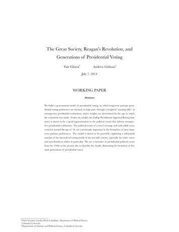
Center in advance of the 2012 election found relatively con-provide a historical narrative of presidential approval over thesistent presidential voting patterns for generations of voters,past half century, emphasizing how particular presidents andwith those generations defined by who was president whenevents had a differential impact on various generations of thethey turned 18 (Kohut et al., 2011: pg. 16).American voting public. We close with discussion.On top of switching the focus to presidential voting, wegeneralize the previously discussed models by allowing the ageData and Preliminary Evidenceweights to vary, in a limited way, by race and region. Giventhe substantial differences between minorities and white peo-Before describing the statistical model in full, it is useful tople, and between Southern and non-Southern whites, it isdescribe the data sources and display some preliminary evi-faulty to assume that the same model of political learningdence. Large sample size is a necessary prerequisite for theshould be applied to all three. Bartels and Jackman, for exam-analysis, because we want the flexibility to define the gener-ple, recognize this and remove white Southerners and Africanational cohorts using individual birth years. American presi-Americans entirely from their analysis. Instead, we incorpo-dential elections benefit from a substantial amount of polling,rate them into the analysis and estimate how well the gener-allowing us to leverage multiple high-quality surveys over theational model fits their observed political development.course of decades.Through this analysis, we find strong and intuitive ageWe combine four major sources of polling: (1) the afore-weights among white voters, particularly non-Southernmentioned ANES cumulative dataset covering the 1952-2008whites. The formation of partisan presidential voting trendstimespan; (2) individually coded Gallup presidential pollingpeaks around the ages of 14-24, with a substantial buildupdata, available from the Roper Center’s iPoll database goingand drawdown in those weights until roughly the age of 40.back to 1952; (3) the 2000, 2004, and 2008 Annenberg Na-The impact of those age weights, combined with different lev-tional Election Studies, large sample surveys giving a partic-els of presidential approval for different birth cohorts, leadularly detailed view of those three elections; and (4) a seriesnaturally to substantial generational trends—to take a promi-of internal campaign polls conducted by Greenberg Quinlannent example, white voters born in 1952, who were mainlyRosner Research over the course of the 2012 election cycle,socialized during the Kennedy and Johnson administrations,to provide coverage for this most recent election. This dataare consistently 5-10 percentage points more likely to sup-was provided for this research by Catalist, LLC, a politicalport Democratic presidential candidates than those born indata vendor7 . For the ANES and Gallup datasets, we only use1968, who were influenced more strongly by the presidenciesdata from presidential election years. After removing missingof Carter, Reagan, and Bush I. The age weights for minori-data8 , we have 306,011 observations in total.ties, in contrast, are much less powerful, suggesting that theirAs a first step, it is helpful to examine the raw data for thepolitical socialization process is somehow different than thatfour most recent elections. The relationship between age andof white voters. Lastly, the data indicate that broad election-presidential vote choice is displayed in the three panels of Fig-by-election changes—normally termed period effects in the lit-ure 1. Here we “control” for race by only displaying data forerature, and quite important when estimating presidentialwhite voters. We describe these graphs in detail to informvote choice as opposed to party identification—are somewhatintuitions and motivate the construction of the model9 .larger for young voters in the impressionable age range thanThe left panel shows the relationship between age and vot-for older voters. A model incorporating all of these factors ex-7 The2012 polls are not publicly available, but the relevant data is availablefor replication purposes on request.8 Variables of interest are presidential vote choice, ethnicity, state of residenceto determine whether white voters live in the South, and age (or, equivalently, birth year, defined here as the year of the survey response minusage).9 For this preliminary analysis, we combine all of the data sources and donot consider house effects or other omitted variables. The full model willmore formally estimate the relationships shown here, and we will describerobustness checks that take omitted variables into account.plains substantially more macro-level variation than a simplemodel accounting for period and race/region effects alone.The paper will proceed by describing the data and statistical model. We then show the model results and how thoseresults can be interpreted to describe the political socialization process for partisan presidential vote choice. Last, we3
204060800.74060800.50.620Age0.4Republican 5Republican Vote0.60.50.40.3Republican Vote2008 McCain VoteLining up by Birth Year0.7Non Monotonicity in Other Elections0.7Non Monotonic Age Curve in 20081990Age197019501930Birth YearFigure 1: Raw data and LOESS curves, indicating the relationship between age and presidential voting preferences among non-Hispanic white voters for the 2000-2012 elections. (L) The relationship is clearly nonmonotonic and quite peculiar in 2008; instead of a linear or even quadratic relationship, the curve changesdirections multiple times. (C) Non-monotonicity is a feature of the other elections as well, though no clear patternis apparent from this graph alone. (R) The true relationship emerges when the curves are lined up by birth yearinstead of age. The peaks and valleys occur in almost identical locations, strongly suggesting a generational trend.ing for the 2008 election. Because we have over 33,000 re-ease interpretability. We notice non-monotonic relationshipssponses for white voters in 2008, we have the statistical powerfor all four of these elections, but the curves are messy and doto separate the data into individual age buckets—each bub-not reveal a clear pattern.ble is a single year of age, with the y -axis indicating level ofFinally, in the right-hand panel, the true insight is revealed.Republican support, in this case for Senator John McCain,Here, we line the curves up by birth year instead of by age, andand the size of each bubble indicating sample size. The fittedthe consistent pattern emerges clearly. All four curves almostcurve is a simple locally weighted regression (LOESS) curve.perfectly in line: the peaks and valleys are nearly identical inWe immediately notice a striking relationship. Republicanevery curve, and, with the exception of the 2008 election, allvote share is neither linearly related to age (as was the casecurves are essentially right on top of each other, especially forin the data from the 1960s), nor is there a simple quadraticvoters born between 1940 and 1970, where the bulk of therelationship, in which middle-aged voters are more likely todata lie. The two peaks in the data occur roughly around thevote for the Republican while both young and old voters arebirth years of 1941 and 1968, with the pro-Democratic valleymore Democratic. Instead, we see a clear non-monotonic re-around 1952. Here, we emphasize that this relationship re-lationship, in which (1) young white voters strongly supportedmains clear and strong over the course of 12 years, measuredthen-candidate Obama, with 18 year olds at about 40% foracross multiple surveys conducted by different organizations,McCain; (2) McCain’s vote grows with age, up to 54% at ageand unaltered by any complicated statistical model. This ap-45; (3) the curve reverses direction, decreasing to 48% for 56-pears to be no statistical artifact.year olds; (4) McCain’s vote climbs again, to it’s peak of 55%Without treading too far into the dreaded age-period-at age 67; (5) the curve takes a final turn, decreasing for the re-cohort framework, it is also important to point out that themainder of the graph and stopping around 50% for the oldest2008 curve is lower than the remaining curves for almost allrespondents.birth cohorts. Recall the overall vote totals for each of theseelections10 . While 2000, 2004, and 2012 were all decided byMoving to the center panel, we overlay a similar curve for10 Thethe 2000, 2004, and 2012 elections, removing the bubbles to4Democratic two-party vote share for the 2000-2012 elections were, in
1007550ObamaBush IIClintonBush an0Roosevelt25Gallup Presidential ApprovalApprove / (Approve Disapprove)19401950196019701980199020002010Figure 2: The Gallup Organization’s Presidential Approval Rating time series, measured from 1937-2012.We use this data to approximate partisan shocks inherent in political events at the presidential level.small margins, 2008 was a relatively robust victory for Demo-dential level. Recall that in the (as yet informally described)cratic candidate Pres. Obama. We and others have com-model, presidential voting choices are informed by a weightedmented on the nature of “uniform swings” in Presidential vot-“running tally” of retrospective evaluations of past presiden-ing (Ghitza and Gelman, 2013), and it certainly seems fromtial performance, with differential weights given to politicalthis data that there was a widespread, if not uniform, swingevents based on when they occurred in an individual’s life-towards Obama in 2008.time. If this is indeed the case, then the Gallup time series isIn sum, the data is strongly suggestive of a model in whichan ideal measurement of those evaluations, even if it only ap-vote choice is generational, at least among white voters. In-proximates the shocks experienced by the public due to eachstead of a purely generational explanation, however, it ap-political event.pears necessary to include period effects to reflect changingeconomic circumstances, cyclical voting habits, candidate-One unfortunate limitation of using this time series, how-centric qualities, and other broad differences between elec-ever, is that despite being one of the longest-running time se-tions. It should be noted, however, that these period effectsries available in the study of American political behavior, itneed not be entirely uniform, a feature we will explore in theis “only” available from 1937 onward. Because the analysismodel.focuses on differential age weights through the entire life cycle, and due to the importance of early life political socializa-Besides individual survey responses, the other main datation suggested in the literature, we are forced to discard anywe use is the Gallup Organization’s long-running Presiden-observations in which we do not have presidential approvaltial Approval Rating time series, displayed in Figure 2. Wedata for the respondents’ entire life span. In other words, weuse this series as an approximation to the partisan shocks thatdrop respondents born before 1937 from the analysis. Thethe public experiences due to political events at the presi-resulting distribution of the data, totaling 201,933 responses,order, 50%, 49%, 54% and 52%; it should be noted that these reflect thevote totals for the full electorate, not for white voters only, as is shown inFigure 1.is separated by election year and then by year of birth in Figure 3. The data cover the 1960-2012 elections, with a strong5
le Size by Birth Year0Number of Survey Responses Included in AnalysisSample Size by Election YearFigure 3: After removing survey respondents born before 1937, the analysis includes 201,933 survey respondents in total, here displayed by election year and year of birth. The data, and thus the analysis, has a strongemphasis towards the most recent four elections, and so it can be interpreted as being weighted towards the contemporary political climate. The data encompass generational cohorts defined by their individual birth year from1937-1994, with at least 1,000 responses for each birth year until 1986.emphasis on the most recent four elections, each having atgether into a single group. It would be preferable to separateleast 25,000 responses. As for generational cohorts defined byAfrican Americans, Hispanics, and other groups, but the databirth year, the data encompass the 1937-1994 cohorts, withfrom earlier years does not always or consistently distinguishat least 1,000 responses for each individual year until 1986between minority groups, forcing us to group minorities to-(the last birth year eligible for the 2004 election).gether for the present analysis.With each respondent indexed according to these characteristics, we can represent the data as J mutually exclusiveStatistical Modelcells, with each cell representing a unique combination ofWe are interested in modeling presidential vote choice bythe three indices. This will help us keep a cleaner notationbirth year cohort over the 1960-2012 elections, distinguish-through the remainder of this section. We label the outcomeing the political socialization mechanism by race and re-variable, presidential vote choice in the observed election, asgion. As such, each survey respondent is indexed by threey and, within any cell j , we label yj as the number of reattributes: (1) his/her birth year cohort c C spondents preferring the Republican candidate, and nj as{1937, 1938, . . . , 1994}, (2) the year of the election t the number of respondents indicating a Republican or DemoT {1960, 1961, . . . , 2012}, and (3) the race/region cratic preference (undecided voters are discarded). The datagroup g G {non-Southern white, Southern white, and model, then, is:minority}. Notice that T includes non-election years—underyj Binomial (nj , θj ) ,this formulation, individuals hold partisan presidential voting(1)tendencies even in non-presidential years, even though theymainly express their preferences through voting in an electionwhere θj is what we want to estimate: the proportion of Re-every four years11 . Also notice that minorities are grouped to-publican presidential support within cell j . Before fully defin-11 Theof latent presidential voting preferences that persist even in non-electionyears.model is, in fact, fit using data observed during presidential electionyears alone. As such, this distinction is a theoretical one facilitating the idea6
ing θj , it is useful to introduce a bit of additional notation.form:For each cell j , xj,i indicates Republican-directional presiden-wi Normal (wi 1 , 1) ,tial approval for age i I {1, 2, . . . , 70} for the birth yearcohort represented in that cell. To construct this, we (1) sub-(3)with no prior expectation on w1 .tract 50% from the Gallup Approval time series, and (2) mul-The purpose of the β term is to estimate the extent to whichtiply the resulting number by 1 when the sitting presidentthe political socialization process implied by the age weightswas a Democrat. The resulting Republican-directional approvalw is different for each race/region group, indexed on g[j]. Awill be positive under two conditions: either a Republicanpriori, we expect minorities to be less impacted by the agepresident has ratings above 50%, or a Democratic presidentweights, due to (a) consistently strong Democratic supporthas ratings below 50%. Conversely, the rating will be nega-among African Americans, and (b) the fact that many His-tive under a popular Democratic or an unpopular Republicanpanic voters may be immigrants, and therefore did not expe-president.rience the political shocks as strongly as white voters who haveThis is a natural way to include directional approval rat-lived in the United States for their entire lives. We do not im-ings into the model, where y 1 indicates Republican sup-pose this expectation through priors in the model, but the βport. As an example, consider the cohort born in 1959. Interms allow us to examine the question. Finally, to keep the1960 (age 1), the average approval rating for the Republi-model identified, the random walk in the w terms is drawncan President Eisenhower was 71%, so xj,1 21%. Inwith a scale parameter σ 1, as shown above, and the w’s1961 (age 2), the presidency flipped to Democratic Presi-themselves are restricted to sum to 1.dent Kennedy, who had an average rating of 88%, yieldingBecause we are modeling presidential vote choice, it is nec-xj,2 1 (88 50) 38%12 .essary to include broad election-by-election period effects,The x’s, then, approximate partisan political shocks thatdenoted αt,g Normal(0, σα ). Notice that the α’s are in-are related to the Presidency. Now that these are specified,dexed by t and g , reflecting potentially different effects bywe define the generational effect on a particular cell:γj βg[j]70 election year and race/regional group. Instead of adding theperiod effects in the same way for all age groups, we general-wi xj,i ,(2)ize the period effect through an interaction term, λg[j ]. Thei 1final period effect Aj for cell j , then, is:where wi indicates the age-specific weight at age i, and βg[j]Aj αt[j],g[j] λg[j] wi[j] αt[j],g[j]() 1 λg[j] wi[j] αt[j],g[j] .reflects the importance of the age-specific weights for eachrace/region group. These are the primary foci of the analy-(4)(5)sis. If the w terms are all roughly the same magnitude, thatwould imply that the simple unweighted “running tally” is anThis generalization is important, because if individuals areappropriate model of retrospective presidential evaluations.more likely to be impacted by political events at a certain age,If, however, they are much higher for some particular agethen it is also reasonable to ask whether election-to-electionrange, then those ages are the foundational ages of presiden-period effects are more pronounced at that impressionabletial political socialization. To structure the analysis a little bit,age as well. We index λ on the group g in cell j , to al-we impose an AR-1 restriction on the w weights, under thelow this interaction to vary by race/region, and we drawexpectation that they take on a somewhat smooth structuralλ Half-Normal (0, σλ ) to normalize the interaction effecttoward zero. Adding these two terms together:12 Twoother notes: (1) The x’s are top-censored at age 70 beca
Jul 06, 2014 · The Great Society,Reagan’s Revolution,and Generations of Presidential Voting Yair Ghitza* Andrew Gelman† July 7,2014 WORKINGPAPER Abstract We build a generational model of presidential voting, in which long-term partisan presi-dential voting preferences are formed,in large pa