WIXLIB

Frames and tensor orientationsmolecularframe M(𝛼, 𝛽, 𝛾)Rtensorframe T% g tensor in eigenframeg eig diag([1.9, 2.0, 2.1])1.90000002.00000002.1000% Euler angles α, β, γ (in radians)abc [10 45 30]*pi/1800.17450.78540.5236% Rotation matrixR 9640.12280.7071rows of R: g axes in molecular framecolumns of R: molecular axes in g frame% g tensor in molecular frameg mol R.'*g .04532.0125% get Euler angles from Reulang(R)*180/pi10.000045.000030.000033

Spin system: Import from ORCA calculationRequesting EPR parameters in ORCAInclude %eprnmr section:%eprnmrgtensor 1Nuclei all H {aiso, adip, aorb, fgrad, rho}endORCA calculationmy.oiftext input fileORCAImport into EasySpinObtain EPR parameters from .prop file:Sys orca2easyspin('my.prop')Visualizationtext output filemy.oof.gbw file.prop filemy.gbwmy.propThanks to Frank Neesereads the .prop fileorcaview34

Spin system: Static broadeningsConvolutional broadeningsisotropic onlyphenomenologically account for line broadeningUnits: mTSys.lwpp [0.2 0.3];Sys.lwpp 0.3;Sys.lw [0 0.1];1st element2nd elementlwpplwSys.lwEndor 0.3;(only salt and saffron), in MHzStrain broadenings(only pepper)GaussianLorentzian (optional)peak-to-peak linewidthfull width at half maximum (FWHM)isotropic or anisotropicUnits: MHzline broadening due to unresolved hf splittings and site-to-site disorderSys.HStrainunresolved hyperfine splittings (MHz)Sys.gStrainSys.AStrainSys.DStraindistribution of g valuesdistribution of A values (correlated with g) (MHz)distribution of D and E (MHz)35

Spin system: Rotational diffusionRotational correlation time(garlic and chili)Sys.tcorr 1e-9;Sys.logtcorr -9;Diffusion tensor c Units: s16R(chili only)Units: 1/sSys.Diff 1e9;Sys.logDiff 9;isotropicSys.Diff [1 2]*1e8;Sys.logDiff [8 8.3];axialSys.Diff [2,2.5,3]*1e8;Sys.logDiff [8.3,8.4,8.5];rhombicSys.DiffFrame [0 20 0]*pi/180; tilt angles fortensor orientation36

Spin system: Ordering potentialOrdering potential coefficients(chili)Expansion coefficients for potential𝐿𝑐𝐿,𝑀 𝐷𝑀0(𝜴)𝑈 𝜴 𝑘B 𝑇𝐿,𝑀Sys.lambda [1 0 0 0 0];First 5 terms: 𝐿, 𝑀 2,0 , 2,2 , 4,0 , 4,2 , (4,4)Frame aligns with diffusion tensor frame37

Static orientational distributionsOrientation of a spin center in the sample:Distribution of orientations of the spin center:Crystals𝜴 (𝜙, 𝜃, 𝜒)𝑃(𝜴)Partially oriented systemsone or several distinctorientations with equalprobabilitiesprobability is varyingfunction of OrderingPowdersall orientations withequal probabilitydefaultSlow motion: "partial MOMD" Slow motion: "MOMD"38

Single crystalsSpecify site splittings via the space or point group of the crystalspace group number and orientation of sites in unit cell site splittingExp.CrystalSymmetry 'P21/m';Exp.CrystalSymmetry 11;space group symbol, Hermann-Mauguinspace group number (between 1 and 230)Not all space group settings are supported.EasySpin requires the third axis of the crystal abc frame to be the unique axis.Exp.CrystalSymmetry 'C2h';Exp.CrystalSymmetry '2/m';point group, Schönflies notationpoint group, Hermann-Mauguin notationUse the point subgroup of the space group, not the local point group of theparamagnetic center.Crystal orientation in the spectrometerthree Euler anglesExp.CrystalOrientation [0 0 0];Exp.CrystalOrientation [0 0 0; 0 pi/2 0];orientation of a crystaltwin crystal39

, Sys.AFrameSys.DFrame, Sys.QFrameSys.eeFrame, Sys.DiffFrameLabframeCrystalframeMolecularframexL, yL, zLxC, yC, zCxM, yM, zMzL along static field (B0)xL along mw field (B1)zC along highest crystalsymmetry axisxC along another symmetryaxis perpendicular to zClocal symmetry frameof spin centerTensorframexT, yT, zTaligned withtensor principal axes40

Single crystalsCrystal rotations- specify rotation axis- generate rotated orientations- specify crystal symmetryn [1 0 0];[phi,theta] rotplane(n,[0 pi],31);Exp.Orientations [phi;theta];Exp.CrystalSymmetry 'P21212';Opt.Output 'separate';[B,spc] pepper(Sys,Exp,Opt);stackplot(B,spc);41

Powder spectra: Orientational averagingEasySpin computes powder spectra by default.Number of orientations10 5 3 2 Opt.nKnots gives the orientationalresolution in terms of number oforientations between θ 0 (north pole) and θ 90 pt.nKnots 10; 10 31;3 91;1 361; 0.25 901; 0.1 1 0.25 The more orientations, the- smoother the spectrum- longer the computation time42

Powder spectra: orientational averaging"Simulation grass"simple summationEasySpin method(projection)absorption1 3 6 first harmonic10 pepper, salt, saffron: Opt.nKnots43

Partially oriented systemsOrientational distribution𝑃 𝜴 exp [ 𝑈 𝜴 /𝑘B 𝑇]Orientational potential𝜆𝐿𝐾 𝑌𝐾𝐿 (𝜴)𝑈 𝜴 𝑘𝐵 𝑇𝐿,𝐾3cos 2 1U ( Ω) kBT 2Predefined potential in EasySpin:Exp.Ordering 2;Custom potential in EasySpin:Exp.Ordering @(ph,th) cos(3*th). 2;absorptionfirst harmonic–252044

cw EPR: a simple exampleSysCu.g [2 2.2];SysCu.lwpp 1;SysCu.Nucs 'Cu';SysCu.A [50 400];ExpX.mwFreq 9.5;ExpX.Range [270 360];pepper(SysCu,ExpX);45

Field sweeps and frequency sweepsField sweepFrequency sweepSys.g [2.05 2.3];Sys.Nucs '63Cu';Sys.A [40 300];Sys.g [2.05 2.3];Sys.Nucs '63Cu';Sys.A [40 300];Sys.lwpp 1;Sys.lwpp 1;% mTExp1.mwFreq 9.5;Exp1.Range [250 360];pepper(Sys,Exp1); % GHz% mT% MHzExp2.Field 350;Exp2.Range [7 10];% mT% GHzpepper(Sys,Exp2);Field sweep: use Exp.mwFreq and Exp.RangeFrequency sweep: use Exp.Field and Exp.RangeIf Exp.range is omitted, EasySpin automatically determines rangeUnits for Sys.lw and Sys.lwpp different for field and frequency sweepsWorks equally for pepper, chili, garlic and all theory levelsField sweep gives first-harmonic, frequency sweep absorption spectrum46

Matrix diagonalization vs. perturbation theoryMatrix diagonalization arbitrary number of electron andnuclear spins general spin Hamiltonian all transitions always exact- slowalways ok!2nd-order perturbation theory- for one electron spin only(S 1/2 and S 1/2)- neglects some Hamiltonian terms- only allowed transitions- accurate only for small A and D many nuclei possible fastuse with care!S 1/2, 63Cu, 2x 14NOpt.Method 'matrix'Opt.Method 'perturb'8.4 s0.08 s47

Energy level diagramsPlotting of energy level n systemorientation'x', 'y', 'z', or angles [𝜙, 𝜃]Rangefield range (mT)[minB0 maxB0]mwFreq microwave frequency (GHz)optional(color indicated allowed/forbidden)Calculation of energy level diagrams without plotting:E levels(Sys,Ori,Range,mwFreq)48

Slow-motion regime simulationsEasySpin implementsFreed's SLE solverRotational dynamicsRotational correlation timeSys.tcorr 1e-9;Sys.tcorr [1 2 10]*1e-9;isotropicanisotropic (axial or rhombic)Rotational diffusion tensorSys.Diff 1e-9;Sys.Diff [1 2 2]*1e-9;isotropicanisotropic (axial or rhombic)Partial orderingOrdering potentialSys.lambda [3 1 0 0 0];potential coefficientsPowders vs. single orientationPowder spectrum (MOMD) by defaultSingle-orientation spectrum: use Exp.CrystalOrientation49

Slow-motion regime simulationsOrientational basis set𝐿Wigner functions 𝐷𝐾,𝑀(𝜙, 𝜃, 𝜒)Maximum values for even L, odd L, K and M:Opt.LLKM [12 0 6 6];The slower the motion and the more anisotropic the spectrum, the largerthese values have to be to produce artifact-free spectra.50

Least-squares fitting: Overviewexperimental spectrumyexpResidualsri f ( yi ,exp ) f ( yi ,sim ( p))nSum of squares ri 22i 1rmsd 2 / NThe global minimum is very difficult to locate!a local minimummodel simulation, ysimDeath Valleythe global minimumDead Sea shore51

Least-squares fitting: MethodsEasySpin does not use analytical derivativesMonte CarlosimplexLev/MargridGlobal methods(search all over the place)- Monte Carlo- genetic algorithms- simulated annealing- tree and grid searchesLocal methods(downhill into valley from a starting point)- Nelder-Mead simplex- Levenberg-Marquardt- NL2SOL, NL2SNO- PowellHybrid methods1) global method to locate promising region(s)2) local method to zero in on minimumAvailable in EasySpin:global methods:- grid search- genetic algiorithm- Monte Carlolocal methods:- Levenberg-Marquardt- Nelder-Mead simplexhybrid methods52

Least-squares fitting: esfitOne interface for all simulation functions.experimental spectrumsimulation parameters[SysFit,spcFit] simulation function(1) Central values of parametersSys0.g [2.008 2.006 2.003];Sys0.Nucs '14N';Sys0.A [16 16 86];Sys0.logtcorr -8.5;spin systemparameter variationsettings forfitting algorithms(2) Allowed variation of parametersone parameter, for 1D searchVary.logtcorr 1;two parameters, for 2D searchVary.logtcorr 0.2;Vary.g [0, 0, 0.0005];No limit on number of parameters, but the more parameters the slower the fitting.53

Least-squares fitting: Multiple componentsOne componentone spin system. esfit('pepper',expspc,SysA,VaryA,,Exp,.)one spin systemparameter variationTwo componentstwo spin systems. p,.)two spin systemparameter variationsWeights in SysA.weight, SysB.weight, VaryA.weight, VaryB.weight.54

Least-squares fitting: SettingsChoosing the algorithm:FitOpt.Method'simplex' Nelder/Mead simplex (default)'levmar' Levenberg/Marquardt'montecarlo' Monte Carlo'genetic' genetic algorithm simplex'grid' grid search simplex'fcn' use spectrum'int' use integralExample:FitOpt.Method 'simplex int'Knowing when to tion tolerance for chi-squaredtermination tolerance for parameter stepmaximum runtimeeach algorithm has different additional parameters55

Least-squares fitting: GUIset method, target, scalingstart/stopcurrent andbestparametersetsblack: datagreen best fitred: current simulationerrorprogresslist of stored parameter sets56

Least-squares fitting: Quality of fitQuality of fit: How deep is the minimum?indicators:- maximum/mean/standard deviation of residuals- residual index R- correlation coefficient of experimental andsimulated spectrum- eye expertisecompare to noise level σ:- max/mean residual σaccurate fit, only random errors in experimental data- max/mean residual σinaccurate fit, systematic errors in simulated spectrumno convergence or wrong modelError of parameters: How steep are the the walls?sensitivity of chi-square to change of parameter values57

Least-squares fitting: Best practicesBefore you start fitting- Baseline correct the spectrum; smooth the spectrum if too noisy.- Choose a physically reasonable model (number of spins, tensors, etc).- Keep the number of fitting parameters as small as possible.- Find good starting parameters by (1) analyzing your spectrum thoroughly,(2) studying literature of similar systems, and (3) using theoretical estimates.- Narrow down the parameter ranges as much as possible.EasySpin (or any other program) cannot find the minimum- if you are too far off initially.- if the parameter ranges are too large or too small.- if there are too many parameters.- if the model is wrong.- if there is too much noise or a non-flat baseline in the spectrum.After convergence- Estimate the goodness-of-fit at the global minimum. It might still be bad.- Look how sensitive the goodness-of-fit is to changes in parameters.- Even the best minimum you find might be physically incorrect.- The global minimum might not be the real minimum due to noise effects.58

Pulse EPR: A first exampleclearSys.Nucs '1H';Sys.A [2 4];Exp.Field 350;Exp.Sequence '2pESEEM';Exp.tau 0.0001;Exp.dt 0.012;Exp.nPoints 501;saffron(Sys,Exp);59

Pulse EPR: OverviewSimulation function: saffronPre-defined pulse sequenceExp.Sequence '2pESEEM';Exp.Sequence '3pESEEM';Exp.Sequence '4pESEEM';Exp.Sequence 'HYSCORE';Exp.Sequence 'MimsENDOR';TimingsExp.tau 0.120;Exp.dt 0.008;Units: μsEcho-detected field sweep?Simulate cw EPR spectrum withpepper, using Exp.Harmonic 0.What it supports- hard and soft pulses- several nuclear spins- high electron spin- user-defined pulse sequences- orientation selection built-in- data processing built-in60

Pulse EPR: Basic experimental settingsMagnetic field (in mT)Exp.Field 350;Spectrometer frequency (in GHz)Exp.mwFreq 9.5;Only needed for orientation selection.Number of pointsExp.nPoints 201;1D and 2DExp.nPoints [64 201]; 2DExcitation bandwidth (in MHz)Exp.ExciteWidth 100;Only needed for orientation selection.If not given, EasySpin uses default values.Pulse experimentDwell time (in μs)Exp.dt 0.008;1D and 2DExp.dt [0.008 0.012]; 2DThis has to be given for ESEEM experiments.Exp.Sequencefor pre-defined pulse experimentsExp.Flip, Exp.Inc, Exp.t, Exp.tpfor user-defined pulse experimentsFrequency range (in MHz)Exp.Range [0 30];This has to be given for ENDOR experiments.61

Pulse EPR: Pre-defined sequencesTwo-pulse ESEEMExp.Sequence '2pESEEM';Exp.tau 0.080;Three-pulse ESEEMExp.Sequence '3pESEEM';Exp.tau 0.100;Exp.T 0.080;HYSCOREExp.Sequence 'HYSCORE';Exp.tau 0.172;Exp.t1 0.08;Exp.t2 0.08;Mims ENDORExp.Sequence 'MimsENDOR';Exp.tau 0.100;Exp.Range [0 30];all times and delays in microseconds62

Pulse EPR: T1 and T2 relaxationRelaxation time constantsExp.T1T2 [10 2];(time for fall-off to 36.8%)first element: T1second element: T263

Pulse EPR, ENDOR: Orientation selectionOrientation/transition selection1. large anisotropies, wide EPR spectrum2. limited excitation bandwidth of mw pulsesParameters necessaryExp.ExciteWidth 100;(Gaussian FWHM, in MHz)Exp.mwFreq 9.5;(has to be given, in GHz)64

Pulse EPR: S 1/2Set electron spinSys.S 1;Sys.S 5/2;Sys.S 7/2;Set zero-field interactionSys.D -200;Sys.D [-130 -80 210];What to remember- flip angles are different for differenttransitions- optimized echo amplitude might notcorrespond to 90 flips for any transition- often strong orientation selection- nuclear frequencies strongly dependon mS65

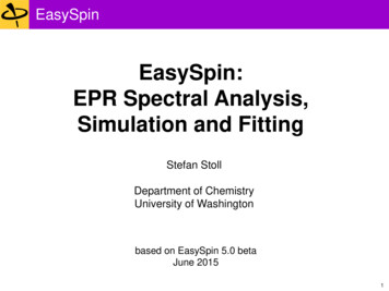
Pulse EPR: S 1/2, many nucleiMn(II)(Im)6S 5/2, I 5/2, and six I 1 (26244 spin states)simulated single-crystal HYSCORE, ideal pulses (6 seconds)66

Pulse EPR: User-defined pulse experimentsFields needed for a user-defined experimentExp.Flippulse flip angle in multiples of 90 Exp.Incincrementation scheme (0 const., 1 first dim., 2 second dim.)Exp.tinitial delays, in microsecondsExample: Two-pulse ESEEMExp.Flip [1 2];Exp.Inc [1 1];Exp.t [0 0];Example: 2D three-pulse ESEEMExp.Flip [1 1 1];Exp.Inc [1 2 1];Exp.t [0.112 0 0.112];Example: HYSCOREExp.Flip [1 1 2 1];Exp.Inc [0 1 2 0];Exp.t [0.1 0 0 0.1];180 90 τ90 constt1t2dim1dim290 τechoconst67

Pulse EPR: Transfer pathways and filters90 90 90 τElectroncoherenceorderT 1 or -10 (α or β)Pathways with detectable echo- equal times in and in –- ending in –Examples:two-pulse ESEEMthree-pulse ESEEMHYSCOREDONUT-HYSCORErefocused primary( -)( α-), ( β-)( αβ-), ( βα-)( αβα-), ( βαβ-)(- -)Pathway filter in EasySpin:three-pulse ESEEM:Exp.Filter '.a.'five-pulse ESEEM: Exp.Filter ' .';τ-1, 1Echo pathways:( α-), ( β-)(-α ), (-β )Pathway filter in EasySpin:Exp.Filter one character per delay' ' 1'-'-1'a'0 (α)'b'0 (β)'.'anything'0'0 (α or β)'1' or Exp.Filter '.a.'Exp.Filter ' .';68

Pulse EPR: Soft (real, non-ideal) pulsesSoft pulses in user-defined sequencesExp.tplength of pulsesExample: HYSCOREExp.Flip [1 1 2 1];Exp.Inc [0 1 2 0];Exp.t [100 0 0 100]*1e-3;Exp.tp [10 10 20 10]*1e-3;Units: μspulse k 1pulse kExp.t(k)Delay values in Exp.t:between end of one pulseand beginning of nextSoft pulses: Offset integration neededOpt.lwOffset width of offset distribution, in MHz(about 1/tp of first pulse; typically 100 MHz)Opt.nOffsets number of integration points (typically 10-30)Soft pulses are not possible with pre-defined sequences!69

Pulse EPR: ENDORSpecifying ENDORExp.Sequence 'MimsENDOR';Exp.Range [135 155]; frequency range (in MHz)Exp.tau 0.100;What to think about- saffron does not (yet) takehyperfine enhancement intoaccount (in contrast to salt)- ENDOR spectrum is simulatedas sum over nucleiENDOR linewidth (in MHz) stick spectrum is convoluted with lineshapeSys.lwEndor 0.1;Gaussian FWHMSys.lwEndor [0.1 0.2];[Gaussian FWHM, Lorentzian FWHM]70

Pulse EPR: Some optionsProduct ruleOpt.ProductRule 0;Opt.ProductRule 1;product rule off (default)product rule on, faster for 3 nucleiHYSCORE log plotOpt.logplot 0;Opt.logplot 1;linear coloring of intensities (default)logarithmic coloring of intensities, gives more detailProcessing optionsOpt.Window 'ham';Opt.ZeroFillFactor 2;apodization window, applied before FFTfactor for zero filling before FFT71

Pulse EPR: Theoretical background1. Hamiltonians- Set up Hamiltonian HS for spins other th

Data import and export eprload reads data from Bruker spectrometers ESP: .spc/.par, BES3T: .DTA/.DSC also loads experimental parameters supports ActiveSpectrum, magnettech and Adani spectrometers load load data stored in Matlab format (.mat) textread reads text (ASCII) data xlsread reads