Transcription
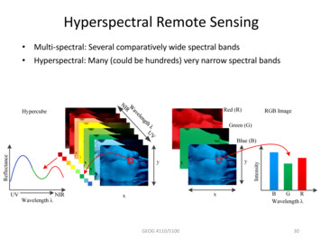
Remote Sensing of Environment 183 (2016) 82–97Contents lists available at ScienceDirectRemote Sensing of Environmentjournal homepage: www.elsevier.com/locate/rseUnderway spectrophotometry along the Atlantic Meridional Transectreveals high performance in satellite chlorophyll retrievalsRobert J.W. Brewin a,b,⁎, Giorgio Dall'Olmo a,b, Silvia Pardo a, Virginie van Dongen-Vogels c, Emmanuel S. Boss daPlymouth Marine Laboratory (PML), Prospect Place, The Hoe, Plymouth PL1 3DH, UKNational Centre for Earth Observation, PML, Plymouth PL1 3DH, UKUniversity of Technology Sydney, Plant Functional Biology & Climate Change Cluster, Sydney, AustraliadSchool of Marine Sciences, University of Maine, Orono, Maine 04469-5741, USbca r t i c l ei n f oArticle history:Received 20 December 2015Received in revised form 4 May 2016Accepted 14 May 2016Available online xxxxKeywords:PhytoplanktonOcean colourRemote sensingChlorophyllValidationAtlantic Oceana b s t r a c tTo evaluate the performance of ocean-colour retrievals of total chlorophyll-a concentration requires direct comparison with concomitant and co-located in situ data. For global comparisons, these in situ match-ups should beideally representative of the distribution of total chlorophyll-a concentration in the global ocean. The oligotrophicgyres constitute the majority of oceanic water, yet are under-sampled due to their inaccessibility and under-represented in global in situ databases. The Atlantic Meridional Transect (AMT) is one of only a few programmes thatconsistently sample oligotrophic waters. In this paper, we used a spectrophotometer on two AMT cruises (AMT19and AMT22) to continuously measure absorption by particles in the water of the ship's flow-through system.From these optical data continuous total chlorophyll-a concentrations were estimated with high precision andaccuracy along each cruise and used to evaluate the performance of ocean-colour algorithms. We conductedthe evaluation using level 3 binned ocean-colour products, and used the high spatial and temporal resolutionof the underway system to maximise the number of match-ups on each cruise. Statistical comparisons show asignificant improvement in the performance of satellite chlorophyll algorithms over previous studies, withroot mean square errors on average less than half ( 0.16 in log10 space) that reported previously using globaldatasets ( 0.34 in log10 space). This improved performance is likely due to the use of continuous absorptionbased chlorophyll estimates, that are highly accurate, sample spatial scales more comparable with satellite pixels,and minimise human errors. Previous comparisons might have reported higher errors due to regional biases indatasets and methodological inconsistencies between investigators. Furthermore, our comparison showed anunderestimate in satellite chlorophyll at low concentrations in 2012 (AMT22), likely due to a small bias in satellite remote-sensing reflectance data. Our results highlight the benefits of using underway spectrophotometricsystems for evaluating satellite ocean-colour data and underline the importance of maintaining in situ observatories that sample the oligotrophic gyres. 2016 The Authors. Published by Elsevier Inc. This is an open access article under the CC BY /).1. IntroductionPhytoplankton are an essential component of the ocean, modifyingits biological, chemical and physical environment. The majority oflight absorbed by phytoplankton is transferred to heat, which can modify the temperature and physical structure of the water column(Sathyendranath, Gouveia, Shetye, Ravindran, & Platt, 1991; Zhai,Tang, Platt, & Sathyendranath, 2011), with a smaller component usedin photosynthesis, the conversion of inorganic carbon (carbon dioxide)to organic carbon. Photosynthesis by phytoplankton is responsible forroughly half of net primary production on Earth (Longhurst,⁎ Corresponding author at: Plymouth Marine Laboratory (PML), Prospect Place, TheHoe, Plymouth PL1 3DH, UK.E-mail address: robr@pml.ac.uk (R.J.W. Brewin).Sathyendranath, Platt, & Caverhill, 1995), helping to modulate thetotal CO2 concentration in water and its pH, influencing CO2 air-seagas exchange, carbon cycling and consequently Earth's climate. Organiccarbon produced by phytoplankton is made available to most marinespecies as an energy source, and ultimately, influences global fishcatch (Chassot et al., 2010). In addition to carbon, phytoplankton contribute to the biogeochemical cycling of a variety of climatically-important elements, such as silica, nitrate and phosphate. It is for thesereasons phytoplankton are recognised as an Essential Climate Variablein the implementation plan of the Global Climate Observing System(GCOS, 2011).Total chlorophyll-a concentration (hereafter denoted chlorophyll),refers to the sum of key photosynthetic pigment concentrations including: monovinyl chlorophyll-a; divinyl chlorophyll-a; and chlorophyllidea (Brotas et al., 2013; Claustre et al., 2004). Partly due to difficulties 4257/ 2016 The Authors. Published by Elsevier Inc. This is an open access article under the CC BY license (http://creativecommons.org/licenses/by/4.0/).
R.J.W. Brewin et al. / Remote Sensing of Environment 183 (2016) 82–97measuring phytoplankton carbon biomass, chlorophyll is used as a simple proxy of phytoplankton biomass (acknowledging biomass-independent changes in chlorophyll can occur from variations in light andnutrients), as it can be routinely estimated in situ (e.g. fluorometrically,using High Performance Liquid Chromatography (HPLC) or absorptionline height) or through satellite remote-sensing of ocean colour (O′Reilly et al., 1998). Collectively chlorophyll in phytoplankton cells has ahuge impact on ocean colour, visible from outer space.Since the launch of the NASA Coastal Zone Color Scanner (CZCS) in1978, and subsequent ocean-colour satellite missions (e.g. the OceanColor and Temperature Sensor (OCTS), the Sea-viewing Wide Field-ofview Sensor (SeaWiFS) of NASA; the Medium Resolution Imaging Spectrometer (MERIS) of ESA; two Moderate Resolution Imaging Spectro-radiometers (MODIS-Aqua and MODIS-Terra) of NASA; and the NASANOAA Visible Infrared Imager Radiometer Suite (VIIRS)), blue-to-greenratios of water reflectance and model-based algorithms have been developed to derive chlorophyll from satellite ocean-colour data. The synopticcoverage, quality and continuity of satellite chlorophyll data has led tomany scientific advances (see McClain, 2009, for a review on this topic),and it is now widely regarded as the main source of data for assessing recent and future change in pelagic ecosystems (Siegel & Franz, 2010).Despite these advances, our understanding of the accuracy and precision of ocean-colour chlorophyll data has been impeded by the limitednumber of, and geographic coverage of, in situ measurements co-incident with the satellite data (O′Reilly et al., 1998). Relative to other satellite-derived oceanic variables, such as sea-surface temperature (e.g.see Table 3 of Merchant et al., 2014), the number of in situ chlorophyllmeasurements co-incident with the satellite data is low. In addition tobeing limited in number, the distribution of in situ data available isoften biased toward coastal and eutrophic waters, with limited dataavailable in the remote oligotrophic waters, despite representing themajority of the surface ocean (Werdell & Bailey, 2005).The Atlantic Meridional Transect (AMT) is a multidisciplinary programme designed to undertake biological, chemical, and physical measurements across a transect of N 12,000 km through the centre of theAtlantic Ocean, ranging from the eutrophic shelf seas and upwelling systems, to the mid-ocean oligotrophic gyres (Aiken et al., 2000; Robinsonet al., 2006). Established in 1995, the programme is now in its 20th year(Rees et al., 2015), having completed (to date) 25 cruises. It was originally conceived to test and ground truth satellite algorithms of oceancolour (in particular the SeaWiFS sensor; Hooker & McClain, 2000) asthe transect crosses a wide range of ocean provinces and conditions,and importantly, crosses the sparsely sampled oligotrophic gyres. Measurements collected on AMT have contributed to global bio-opticaldatasets used for satellite algorithm development and validation (O′Reilly et al., 1998; Werdell & Bailey, 2005), and have been used to assessthe performance of satellite ocean-colour chlorophyll retrievals (Aikenet al., 2009; Brewin et al., 2010; Brewin, Sathyendranath, Jackson, etal., 2015). AMT is widely recognised as an ideal platform to evaluate satellite ocean-colour data (Aiken & Hooker, 1997; Hooker & McClain,2000; Rees et al., 2015).Traditionally, satellite chlorophyll data has been validated using coincident discrete point measurements of chlorophyll, such as that acquired through HPLC or through fluorometric chlorophyll extraction.When comparing co-incident in situ point measurements with the satellite data, errors can occur due to vast differences in the observationalscales of the two types of measurements. Discrete in situ measurementsof chlorophyll typically represent volumes of sea water of the order of5 l or less, whereas satellite ocean-colour pixels are typically between1 km and 4 km in size, which if one assumes an optical depth of 10 m(often much deeper in clear waters), equates to a volume of water inthe region of 1 1010 and 16 1010 l. Furthermore, the spatial variability within a satellite pixel is very difficult to sample using discrete pointmeasurements.One option to address this mismatch in spatial scales between satellite and discrete point measurements is by using continuous in situ data83collected by a moving ship. Since the 1930′s plankton measurementshave been collected using the Continuous Plankton Recorder towed onresearch vessels and voluntary ships, and have been used for comparison with satellite ocean-colour data (Batten, Walne, Edwards, &Groom, 2003; Brewin et al., 2011; Raitsos, Reid, Lavender, Edwards, &Richardson, 2005). Continuous chlorophyll data derived from a lidarfluorosensor on a moving research vessel have also been comparedwith ocean-colour chlorophyll data over wide spatial scales (Barbini,Colao, Fantoni, Fiorani, & Palucci, 2003; Barbini et al., 2004). A commonapproach to collecting continuous in situ chlorophyll measurments isthrough calibrated in vivo fluorescence data collected by sampling surface water from the flow-through system of a moving ship (Lorenzen,1966). This approach has been used to validate ocean-colour data incoastal (Folkestad, Pettersson, & Durand, 2007; Harding, Magnuson, &Mallonee, 2005; Petersen, Wehde, Krasemann, Colijn, & Schroeder,2008) and shelf regions (Hu et al., 2003, 2005; Zhang et al., 2006), andhas demonstrated the importance of validating a satellite pixel usingmultiple samples in heterogeneous conditions (Hu, Nababan, Biggs, &Muller-Karger, 2004). Yet, this approach has its caveats. For instance,the fluorescence yield can vary between species of phytoplankton(Kiefer, 1973b; Strickland, 1968) and within a single species subjectedto different environmental conditions (Kiefer, 1973a; Slovacek &Bannister, 1973). In vivo fluorescence in surface waters can also be affected by non-photochemical quenching during daytime (e.g. Cullen &Lewis, 1995). These problems impact the accuracy and precision of thein situ chlorophyll data, particularly in the oligotrophic gyres (Strass,1990).Recently, techniques have been developed to continuously measurethe inherent optical properties of particles in surface sea water sampledby the flow-through system of a moving ship (Boss et al., 2013;Dall'Olmo, Boss, Behrenfeld, & Westberry, 2012; Dall'Olmo, Westberry,Behrenfeld, Boss, & Slade, 2009; Dall'Olmo et al., 2011; Koponen et al.,2007; Slade et al., 2010; Westberry, Dall'Olmo, Behrenfeld, & Moutin,2010). Using these techniques, chlorophyll concentration can be estimated with remarkable accuracy and continuously, using particulateabsorption measurements and the line-height of the absorption peakat red wavelengths (Boss, Collier, Larson, Fennel, & Pegau, 2007;Dall'Olmo et al., 2012; Davis, Moore, Zaneveld, & Napp, 1997;Westberry et al., 2010). These techniques have been used to evaluateocean-colour data (Brewin, Raitsos, et al., 2015; Werdell, Proctor, Boss,Leeuw, & Ouhssain, 2013) and have the potential to overcome some ofthe caveats of estimating chlorophyll using in vivo fluorescence.In this paper, we use an optical set-up on two AMT cruises (AMT19and AMT22) to continuously measure chlorophyll concentration fromthe ship's flow-through system. The chlorophyll datasets are thenused to evaluate the performance of satellite chlorophyll algorithmson different ocean-colour sensors.2. Methodology2.1. Statistical testsTo test the performance of satellite chlorophyll algorithms we used aseries of univariate statistical tests commonly used in comparisons between modelled and in situ data (e.g. Brewin, Sathyendranath, Müller,et al., 2015; Doney et al., 2009; Friedrichs et al., 2009), including: thePearson correlation coefficient (r); the root mean square error (Ψ);the average bias between model and measurement (δ); the unbiasedroot mean square error (Δ); the slope (S) and intercept (I) of a Type-2regression; and the percentage of possible retrievals (η). For S and I,we used Type-2 regression (Glover, Jenkins, & Doney, 2011, MATLABfunction lsqfitma.m). The equations used for each of these statisticaltests are provided in Table 1. All statistical tests were performed inlog10 space, considering chlorophyll is approximately log-normally distributed in the ocean (Campbell, 1995, see also Fig. 3b).
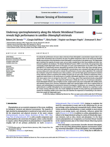
84R.J.W. Brewin et al. / Remote Sensing of Environment 183 (2016) 82–97Table 1Summary of statistical tests used in the study.SymbolDescriptionEquationarPearson correlation coefficientNMNEN1CMC Ei ðN1 m¼1 C m Þi ðN j¼1 C j Þ1 ½ N 1 ½2 1 22 1 2NNEi¼11E11NNMfN 1 n¼1 ½C n ðN o¼1 C o Þ g1fN 1 k¼1 ½C Mk ð l¼1 C l Þ gΨRoot mean square errorδBiasΔUnbiased root mean square errorSSlope of Type-2 regressionbIηNN21 2½N1 ðC Ei C Mi Þ i¼1NEM1N ðC i C i Þi¼1bIntercept of Type-2 regressionPercentage of possible retrievals2 1 2N1 N1 N MðN1 f½C Ei ð C Ej Þ ½C Mi ð C k Þ g ÞN j¼1N k¼1i¼1C E ICMEC SCMNENM100aC denotes the variable (chlorophyll concentration) and N is the number of samples with both estimated and measured data. The superscript E denotes the estimated variable (e.g. usingsatellite data) and the superscript M denotes the measured variable (e.g. measured in situ).bType-2 regression between CM and CE (where CE CMS I) was used to derive S and I.2.2. Underway optical samplingAMT19 and AMT22 underway data were collected on board the RRSJames Cook from the 14th of October to the 28th of November 2009, andthe 15th October to the 20th of November 2012, respectively. Bothcruises followed a very similar cruise track, spanning 50 N to 50 S(Fig. 1).On both cruises, optical instruments were attached to the ship'sclean flow-through system, continuously pumping seawater from anominal depth of about 5 m. The methods of Dall'Olmo et al. (2009),Slade et al. (2010) and Dall'Olmo et al. (2012) were followed, which involved first passing water through a Vortex debubbler, then either passing water directly through the optical instruments (50 min for everyhour) or diverting seawater through a Cole Parmer 0.2 μm-cartridge filter (for 10 min every hour), the later used to provide a baseline for particulate absorption measurements. Either a WET Labs AC-Shyperspectral spectrophotometer (hyperspectral between 400 and 750 nm, with a spectral resolution of 5 nm and a band pass of15 nm), or a WET Labs AC-9 (nine wavelengths between 412 and715 nm, with a band pass of 10 nm) were used to measure spectral absorption. Spectral particulate absorption (ap(λ)) were calculated bysubtracting the 0.2 μm filtered measurements from the unfilteredmeasurements, providing calibration-independent estimates of ap(λ)accounting for instrumental drifts and residual calibration errors. Following Dall'Olmo et al. (2009), data were converted into 1-min medianbins. The 1-min binned data were medians of higher frequency data( 240 measurements): when the ship moves at 18 km h 1 (typically),each 1-min binned average is representative of approximately 0.3 km.For AMT19, an AC-S was used at the beginning of the cruise but after13 days the lamp of the attenuation channel (i.e., C-channel) failed,and an AC9 meter was added to the flow-through system (Dall'Olmoet al., 2012). As the “band pass” of the AC9 is narrower (10 nm) thanthat of the AC-S (15 nm), concurrent AC-9 and AC-S ap(λ) data were calibrated to ensure no systematic bias in ap(λ) between instruments (seeSection 2.1.3 of Dall'Olmo et al., 2012, for further details). For AMT22, aWET Labs AC-S was used during the entire cruise.For both AMT19 and AMT22, discrete water samples (2 to 4 l) werecollected along the transects from the underway flow-through system.The water samples were filtered onto Whatman GF/F filters (nominalpore size of 0.7 μm) and stored in liquid nitrogen. Chlorophyll (C) wasdetermined after the cruise in the laboratory using HPLC analysis.To estimate chlorophyll from the underway optical system, data forap(λ) were extracted at 650, 676 and 715 nm. The phytoplankton absorption coefficient at 676 nm (aph(676)) was then estimated usingFig. 1. (a) Cruise tracks for AMT19 (Oct-Nov 2009) and AMT22 (Oct-Nov 2012) for underway HPLC data; (b) and (c) show the relationship between co-located (20 min time window)aph(676), derived from the underway optical system (OS) and underway HPLC chlorophyll (C), for AMT19 (106 samples) and AMT22 (176 samples) respectively; (d) and (e) showchlorophyll (C) from HPLC and the underway optical system (OS) with latitude for the two cruises; (f) shows the relationship between HPLC and OS-inferred chlorophyll; and (g)absolute log10-transformed difference between HPLC and OS-inferred chlorophyll.
R.J.W. Brewin et al. / Remote Sensing of Environment 183 (2016) 82–97the line height method of Davis et al. (1997) as modified by Boss et al.(2007), such that aph ð676Þ ¼ ap ð676Þ 39 65ap ð650Þ þ 26 65ap ð715Þ :ð1ÞTo convert aph(676) into chlorophyll concentrations (C), we extractedconcurrent data on aph(676) from the optical system to that of the discreteHPLC chlorophyll data. The aph(676) data were averaged in log10 spaceover a 20-min period centered on the time the discrete HPLC water samples were collected ( 10 min), then back-transformed. We then fitted anon-linear relationship (Bricaud, Babin, Morel, & Claustre, 1995; Bricaud,Morel, Babin, Allali, & Claustre, 1998) between aph(676) and C, such thatC ¼ Aaph ð676ÞB :ð2ÞThe parameters A and B were determined for each cruise separately,by fitting Eq. (2) using HPLC chlorophyll and corresponding data onaph(676) from the optical system. For AMT19, estimates of A and Bwere 88 and 1.02 (N 106), respectively. For AMT22, A and B were62 and 0.99 (N 176), respectively. In both cases, the slope of thepower-law function (B) was not significantly different from 1.0, suggesting a linear relationship between aph(676) and C along the twoAMT cruise tracks, in contrast to previous studies using global datasets(e.g. Brewin, Devred, Sathyendranath, Hardman-Mountford, &Lavender, 2011; Bricaud et al., 1995, 1998; Werdell et al., 2013). Toabide by the law of parsimony, Eq. (2) was replaced with a linear relationship between aph(676) and C, such thatC ¼ Aaph ð676Þ:ð3ÞThe parameter A was estimated as 80 2.0 and 69 1.3 for AMT19and AMT22 respectively (Fig. 1b and c), where the uncertainties are the95% confidence intervals of the means. Note that the parameter A is influenced not only by the chl-specific absorption coefficient at 676 nm,but also by differences in the optical set-up on the two cruises (e.g. different instruments with different spectral responses). Fig. 1d–g show acomparison of chlorophyll estimated from the optical set-up (Eq. (3))with the corresponding HPLC chlorophyll data. The optical set-up isshown to estimate chlorophyll with very good accuracy along the twoAMT transects. Eqs. (1) and (3) were used to reconstruct chlorophyllfor all ap data collected on AMT19 and AMT22, resulting in 45,171 1min binned chlorophyll samples for AMT19 and 34,934 for AMT22.2.3. In situ hyperspectral radiometryTo aid interpretation of the satellite chlorophyll validation results,we used in situ above-water hyperspectral radiometry data collectedon AMT19 and AMT22. An above-water Hyperspectral Surface Acquisition Remote Sensing System (SATLANTIC HYPERSAS) was installed on afixed pole on the bow of the ship on both AMT19 and AMT22.Hyperspectral downwelling irradiance (Es), sky radiance (Li) andwater-leaving radiance (Lt) were recorded at a number of stationsalong the AMT track. These stations all occurred around local noon,where the ship stopped for CTD profiles. On both cruises, the Es sensorwas pointed toward zenith, with the Li and Lt sensors deployed atfixed angles facing the sky and water respectively ( 40 and 130 respectively from nadir, assuming a horizontal ship). Sensor windowswere regularly cleaned during both cruises with lens paper.Es, Li and Lt were extracted from the HYPERSAS for a 1-h period overthe duration of each station, using SATLANTIC SatView and SatCon software. The HYPERSAS data were processed as follows: On each instrument, a shutter closes periodically to record darkvalues. The Es, Li and Lt data were first dark corrected, by interpolatingthe dark value data in time to match the light measurements for eachsensor, then subtracting the dark values from the light measurementsat each wavelength.85 The Es, Li and Lt were then interpolated to the same set of wavelengths(every 3.5 nm from 350–800 nm), which coincides roughly with thewavelengths of the Es sensor, the instrument with the smallest number of channels. As the three sensors have different integration times and thus collectdata at slightly different time stamps, the Es, Li and Lt data were interpolated to the same set of time stamps, which was selected based onthe sensor with the slowest integration time (typcially the Lt sensor).This resulted in Es, Li and Lt data at the same time and same sets ofwavelengths. For each station, only spectra with a sun zenith angle of b60 , an azimuth angle between either 100 and 170 (centered at 135 35 )were used (Mobley, 1999). Any spectra with negative values at443 nm (which can occur when cleaning the sensor) were removed. To minimise sun glint contamination we exploited the near-infraredportion of the Lt reflectance spectrum which, in open ocean waters,should be close to zero. The statistical distribution of Lt(NIR) data,where NIR represents the average of Lt in the region 750–800 nm, ateach station was analysed and spectra were only retained in thelower 5th percentile of Lt(NIR) (Hooker, Lazin, Zibordi, & McLean,2002). Remote-sensing reflectance (Rrs(λ)) was then computed according toRrs(λ) [Lt(λ) ρLi(λ)]/Es(λ), where ρ was computed for each stationfollowing (Mobley, 2015), using the median wind speed, azimuthangle, and sun zenith angle over the duration of each station, and assuming a viewing angle of 40 . Rrs(λ) data in the near-infrared were computed (averaged in the region 750–800 nm) and subtracted from each spectra, to remove anyadditional contamination by sky and sun glint. For the remaining spectra at each station, remote-sensing reflectanceratios (Rrs(443)/Rrs(547) and Rrs(488)/Rrs(547)) were computed. Median Rrs(443)/Rrs(547) and Rrs(488)/Rrs(547) values were extractedfor each station, after degrading the hyperspectral Rrs data to 11 nmaverages centered on each wavelength, to be consistent withNOMAD data used to parameterise the NASA OC-series of chlorophyllalgorithms (Werdell & Bailey, 2005). To remove noisy station data andmaximise the consistency of the dataset, only station data were usedwhere the maximum coefficient of variation of Rrs(443)/Rrs(547)and Rrs(448)/Rrs(547) was less than 0.15. Finally, chlorophyll data from the optical system were extracted forthe same time period at each station (1 h) and median concentrationswere computed. This resulted in 8 stations on AMT19 and 22 stationson AMT22 with concurrent in situ Rrs(443)/Rrs(547), Rrs(448)/Rrs(547)and chlorophyll.2.4. Satellite ocean-colour datasetsWe conducted our ocean-colour evaluation using daily, level 3, 4 kmbinned satellite ocean-colour products. The choice to use level 3 (4 km)ocean-colour products for the evaluation, as opposed to level 2 (1 km)typically used in satellite validation protocols (Bailey & Werdell,2006), stems from: (i) the continuous underway sampling methodused allows for many samples to be collected within a 4 km pixel, to account for the effects of sub-pixel variability over a larger pixel area; (ii)the merged ocean-colour products evaluated here are merged at level 3rather than level 2; and (iii) in a recent user requirements survey(Sathyendranath, 2011), it was found that ecosystem modellers andearth observation scientists using ocean-colour data have a preferencefor level 3 products over level 2. Nonetheless, we investigate the impactof using level 3 data for validation by comparing results with a validation using level 2 data.For the AMT19 period (14th of October to the 28th of November2009), MODIS-Aqua (R2014.0 and R2013.1) and MERIS (processedwith SeaDAS, R2012.1) daily, global, level 3 spectral remote-sensing
nusoidalSinusoidalSinusoidalSinusoidalLevel 3Level 3Level 2Level 3Level 3Level 3Level 3Level 3Level 3Level 3Level 3Level 3Level 3Data acquired from 14th of October to 28th of November 2009 for AMT19, and 15th October to 20th of November 2012 for AMT22.Number of satellite and in situ match-ups used in the evaluation.Satellite data collected at the native resolution of the MERISOC-CCI v1.0OC-CCI v2.0MODIS-AquaMODIS-AquaVIIRSOC-CCI v1.0OC-CCI v2.019191919191919192222222222bDailyDailySwath ailyR2013.1R2014.0R2014.0R2010.0R2012.1Version 3.0Version 1.0Version 2.0R2013.1R2014.0R2014.0Version 1.0Version 47OC3M-547OC3VOC4OC4Standard chlorophyll algorithm usedProductSensorAMTTable 2Information on the satellite datasets used in this study. To minimise effects of sub-pixel variability on the validation, satelliteRrs(λ) data were matched in time (same day of year) and space(latitude and longitude, closest 4 km pixel) with the in situ chlorophyll data for AMT19 and AMT22. When one or more in situsamples were matched to the same satellite pixel, the in situ chlorophyll concentrations were averaged (using log 10 transformation) and considered as a single match-up. Only samples wereused where there were N5 in situ data points within a satellitepixel (Fig. 2a), and where the standard deviation of the in situlog 10 (C) measurements was less than 0.1 ( 95 percentile ofdata, see Fig. 2b). To test for homogeneity of the region surrounding the satellitematch-up, eight other satellite pixels surrounding the centrepixel (total of 9, 3 3) were also extracted from the satellitedata. The coefficient of variation (median coefficient of variationfor Rrs bands between 412 and 555 nm) for each box of nine pixelswas then computed. Match-ups were excluded if the coefficientof variation was N0.15 (Fig. 2c, similar to Bailey & Werdell,2006, acknowledging that they used 5 5 km level 2 data) andwhen b 50% of the pixels were available in the surrounding region. Finally, the average solar zenith angle for the in situ chlorophylldata within each satellite match-up was computed, using thetime and location of in situ data collection. To minmise the timedifference between satellite and in situ data collection, onlymatch-ups with a solar zenith angle b90 were used (Fig. 2d),meaning that only underway data collected during daylighthours were used in the study. Regarding this latter point, thetime difference between satellite and in situ data will vary depending on satellite overpass time, which is different for each satellite. For merged products, this becomes more complicated tocompute, as a merged product contains a combination of information from different satellite sensors, that collect data atVersion/ReprocessingThe following procedure was implemented to ensure high qualitymatch-ups between Level 3 satellite Rrs(λ) and in situ chlorophyll orala resolution2.5. Satellite and in situ match-up procedureaSpatial resolutionProcessing levelProjectionAtmospheric correction algorithm usedNbreflectance Rrs(λ) data were downloaded from the NASA website(http://oceancolor.gsfc.nasa.gov/). Level 3, global, 4 km MERIS oceancolour Rrs(λ) products were also produced using the POLYMER atmospheric-correction algorithm (version 3.0; Steinmetz, Deschamps, &Ramon, 2011) over the AMT19 period. SeaWiFS (R2010.0) level 3,global, 4 km data were produced at Plymouth Marine Laboratory(PML), by re-binning Level 2 SeaWiFS data (acquired from NASA)to a 4 km grid, as the NASA level 3 SeaWiFS products are providedat 9 km. In addition to single-sensor datasets, we also downloadedmerged ocean-colour products from the European Space Agency(ESA) Ocean Colour Climate Change Initiative (OC-CCI) over theAMT19 period. OC-CCI data constitute merged (level 3, 4 km binned)MERIS (POLYMER), MODIS-Aqua and SeaWiFS products, and areavailable at http://www.oceancolour.org/ (Sathyendranath et al.,2012). Both versions 1.0 and 2.0 of the OC-CCI products
lite remote-sensing reflectance data. Our results highlight the benefits of using underway spectrophotometric . Color and Temperature Sensor (OCTS), the Sea-viewing Wide Field-of-view Sensor (SeaWiFS) of NASA; the Medium Resolution Imaging Spec- . Using these techniques, chlorophyll con