142 IEEE GEOSCIENCE AND REMOTE SENSING LETTERS, VOL. PDF Free Download

2y ago

47 Views

1 Downloads

2.37 MB

5 Pages

Report/dmca

Download PDF

Transcription

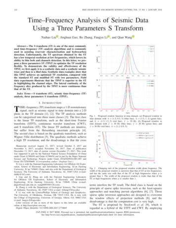
142IEEE GEOSCIENCE AND REMOTE SENSING LETTERS, VOL. 15, NO. 1, JANUARY 2018Time–Frequency Analysis of Seismic DataUsing a Three Parameters S TransformNaihao Liu , Jinghuai Gao, Bo Zhang, Fangyu Li , and Qian WangAbstract— The S transform (ST) is one of the most commonlyused time–frequency (TF) analysis algorithms and is commonlyused in assisting reservoir characterization and hydrocarbondetection. Unfortunately, the TF spectrum obtained by the SThas a low temporal resolution at low frequencies, which lowers itsability in thin beds and channels detection. In this letter, we propose a three parameters ST (TPST) to optimize the TF resolutionflexibly. To demonstrate the validity and effectiveness of theTPST, we first apply it to a synthetic data and a synthetic seismictrace and then to a filed data. Synthetic data examples show thatthis TPST achieves an optimized TF resolution, compared withthe standard ST and modified ST with two parameters. Fielddata experiments illustrate that the TPST is superior to the STin highlighting the channel edges. The lateral continuity of thefrequency slice produced by the TPST is more continuous thanthat of the ST.Index Terms— S transform (ST), seismic time–frequency (TF)analysis, three parameters S transform (TPST).I. I NTRODUCTIONTIME–frequency (TF) transform maps a 1-D nonstationarysignal, such as seismic signal in time domain into a 2-Dplane in the TF domain [1], [2]. The TF analysis methodscan be categorized into three main classes [3]. The first classis the linear TF transform, such as the short-time Fouriertransform (STFT), continuous wavelet transform (CWT),and S transform (ST). The linear TF methods are intuitive,but suffer from the Heisenberg uncertain principle [4].The second class is based on the quadratic transform, such asWigner–Ville distribution [5]. The quadratic methods achievea high TF resolution, and the disadvantage is that the crossManuscript received August 22, 2017; revised October 9, 2017 andNovember 4, 2017; accepted November 20, 2017. Date of publicationDecember 13, 2017; date of current version December 27, 2017. This workwas supported in part by the National Natural Science Foundation of Chinaunder Grant 41390450 and Grant 41390454 and in part by the Major NationalScience and Technology Projects under Grant 2016ZX05024-001-007 andGrant 2017ZX050609. (Corresponding author: Jinghuai Gao.)N. Liu is with the National Engineering Laboratory for Offshore Oil Exploration, School of Electronic and Information Engineering, Xi’an JiaotongUniversity, Xi’an 710049, China, and also with the Department of GeologicalSciences, The University of Alabama, Tuscaloosa, AL 35487 USA (e-mail:lnhfly@163.com).J. Gao and Q. Wang are with the National Engineering Laboratoryfor Offshore Oil Exploration, School of Electronic and InformationEngineering, Xi’an Jiaotong University, Xi’an 710049, China (e-mail:jhgao@mail.xjtu.edu.cn; wqlq668930@126.com).B. Zhang is with the Department of Geological Sciences, The Universityof Alabama, Tuscaloosa, AL 35487 USA (e-mail: bzhang33@ua.edu).F. Li was with the ConocoPhillips School of Geology and Geophysics,The University of Oklahoma, Norman, OK 73019 USA. He is now withthe College of Engineering, University of Georgia, Athens, GA 30602 USA(e-mail: fangyu.li@uga.edu).Color versions of one or more of the figures in this letter are availableonline at http://ieeexplore.ieee.org.Digital Object Identifier 10.1109/LGRS.2017.2778045Fig. 1. Proposed window function in time domain. (a) Proposed window intime domain with (1.5, 0.5, 3) (blue line), (1.5, 1, 3) (green line),and (1.5, 1.5, 3) (red line), f 10 Hz. (b) Proposed window intime domain with f 10 Hz (blue line), f 20 Hz (green line), andf 30 Hz (red line), (1.2, 0.9, 5).Fig. 2. Changing rule of the proposed window width about frequency. Thewidth of the proposed window is narrower than that of ST at low frequencies,and has the same size with that of the ST at high frequencies when p isgreater than 1. The width of the proposed window is wider than that of theST at high frequencies when p is smaller than 1.terms interfere the TF result. The third class is based on theprinciple of sparse spike inversion, such as the least-squaresapproaches and matching pursuit algorithms [6], [7]. Thosesparse spike inversion approaches are designed to overcomethe window effects of projection methods [8], and thedisadvantage is that the computation cost is very high.The ST is proposed by Stockwell et al. [9], which isregarded as a hybrid of the STFT and CWT. By employing1545-598X 2017 IEEE. Personal use is permitted, but republication/redistribution requires IEEE permission.See http://www.ieee.org/publications standards/publications/rights/index.html for more information.

LIU et al.: TF ANALYSIS OF SEISMIC DATA USING A TPST143Fig. 3. Synthetic data example. (a) Noise-free (red line) and noisy (green line) synthetic signals s(t), consisting of three components. Noise-free TF spectraproduced by (b) ST, (c) MST, and (d) TPST. Noisy TF spectra calculated by (e) ST, (f) MST, and (g) TPST.the Fourier transformation kernel, the ST retains the absolutephase information. By using a frequency-dependent windowfunction, it can produce high time resolution at high frequencies and high frequency resolution at low frequencies. Thestandard deviation of the Gaussian function scales inverselywith the frequency, which produces a frequency-dependentresolution for the ST [10]. Also, the ST maintains a directrelationship with the Fourier transform, which is helpful toreconstruct the analyzed signal. However, there is no parameter to adjust the window width of the ST resulting ina poor time resolution at low frequencies and degrade thefrequency resolution at high frequencies. Various modifiedwindow functions were proposed to optimize the TF resolution. Mansinha et al. [11] proposed the 2-D ST and appliedit to the pattern analysis. McFadden et al. [12] proposeda generalized ST (GST) by using an asymmetrical windowfunction. Pinnegar and Mansinha [13] developed another formGST and applied it to determine the P-wave arrival time ina noisy seismogram. Pinnegar and Mansinha [13] used twoprescribed frequency functions to control the scale and theshape of the analyzing window. Li and Castagna [14] proposeda modified ST (MST) with two parameters and employ itto direct hydrocarbon detection. Sejdić et al. [15] improvedenergy concentration in the TF domain by introducing aparameter to the window in the ST.In this letter, we propose a three parameters ST (TPST) andapply it to detect the channels and characterize the channelfeatures. We first briefly review the theory of the standard ST.We then propose to optimize the TF resolution of the ST usinga TPST. The proposed method is first tested by a syntheticsignal and a synthetic seismic trace and then to real seismicdata.II. S T RANSFORMThe ST of a signal s(t) is defined as [9] (t τ )2 f 2 f ST(τ, f ) s(t) e 2 e i2π f t dt2π (1)

144IEEE GEOSCIENCE AND REMOTE SENSING LETTERS, VOL. 15, NO. 1, JANUARY 2018Fig. 4. Seismic synthetic trace example. (a) Reflectivity. (b) Seismic synthetic trace. TF spectra calculated by (c) standard ST, (d) MST, and (e) TPST. Thereare three reflection sets in this model. The first set only contains one reflectivity with a positive magnitude of 0.3. The magnitude of the second reflectionset is 0.3 with the opposite sign. The third reflection set contains two reflectivities with a positive magnitude of 0.3. The time thicknesses of the second andthird pairs are 30 and 40 ms.where t and f are time and frequency variables. τ denotesthe localization of the frequency-dependent Gaussian window.The advantage of the ST over the STFT is that the ST performsa multiresolution of the analyzed signal s(t).According to Parseval’s theorem, (1) can be rewritten in thefrequency domain as 2 2 2π αST(τ, f ) S(α f )e f 2 ei2πατ dα(2) where S(α) is the Fourier transform of s(t). Obviously, takingadvantage of the fast Fourier transform, the ST has a fastimplementation.III. T HREE PARAMETERS S T RANSFORMThe window used in the ST has standard deviation variedover frequency. However, the changing rule of the standarddeviation remains invariable, and this is the main limitationof the ST. To remedy this drawback, a simple improvementcan be obtained by modifying the standard deviation of thewindow in the ST as1(3)δ( f ) p k f m where (k, p, m) are adjustable parameters. k is aparameter defining the mode of the window width. p adjuststhe changing rate of the window width and m controls thetradeoff between the ST and STFT. Based on (3), the TPSTcan be expressed as k f p m (t τ )2 (k f p m)2 i2π f t2TPST(τ, f ) s(t) edt.e2π (4)The width of the proposed window is independent of frequency, and the TPST is degraded into the STFT whenconsidering k 0 and m 1. The TPST approaches thestandard ST when (1, 1, 0).According to Parseval’s theorem, (4) can be rewritten in theFourier domain as 2 2 2π αS(α f )e (k f p m)2 ei2πατ dα.(5)TPST(τ, f ) Note that the three parameters (k, p, m) control the widthand shape of the window function in the time and frequencydomains, by squeezing or stretching it. As a result, thisdistinctly achieves an adaptive and optimized TF resolution.Fig. 1 illustrates the proposed window in time domainfor various parameters and various frequencies, respectively.Fig. 1(a) shows that the time resolution is increasing withincreasing p. Fig. 1(b) illustrates that the time resolutionis increasing with increasing frequency. Thus, our proposedmethod has the capability to improve the time resolution atthe low frequency and compared with the standard ST.

LIU et al.: TF ANALYSIS OF SEISMIC DATA USING A TPST145Fig. 2 shows the varying of the window width withvarying frequencies for a different control parameters set (k, p, m). The window width of the TPST (red line) ismore compact than that of the ST (blue line) at low frequencieswhen p is greater than 1.This phenomenon indicates that theTPST has a higher time resolution than the ST when p isgreater than 1. The window width of the TPST has the samesize with that of the ST at high frequencies. This phenomenonindicates that the TPST has the same time resolution as the ST.The window width of the TPST is wider than that of thestandard ST at high frequencies when p is smaller than 1.This phenomenon indicates that the TPST has an improved frequency resolution when p is smaller than 1. The above featuresindicate that we can obtain an adaptive TF representation withoptimized TF resolution by choosing suitable parameters in theTPST. Note that we optimize the three parameters in the TPSTusing the concentration measure (CM) approach [17] in thisletter. By optimizing the three parameters in the TPST usingthe CM method, we achieve an optimized TF representation.IV. I NVERSION OF T HREE PARAMETERS S T RANSFORMThe window function in the TPST satisfies the admissibilitycondition of unit area as k f p m (t τ )2 (k f p m)22 edτ 1.(6)2π This normalization condition guarantees the energyinversion of the TPST. By integrating the TF spectrum overtime, the relationship between the Fourier spectrum andTF spectrum of the TPST is defined as TPST(τ, f )dτ S( f )(7) where S( f ) is the Fourier transform of s(t). Therefore, theinput signal can be simply reconstructed as s(t) TPST(τ, f )ei2π f t dτ d f .(8) V. S YNTHETIC AND F IELD DATA E XAMPLESIn this section, we apply the TPST to synthetic signalsand field data to compare its performance with the standardST and MST with two parameters [17]. Fig. 3(a) shows acomposited signal s(t) in (9) (red line) containing three slowlyvarying frequency components [14], [15], where the green linedenotes the noisy signal added with Gaussian white noise. TheSNR equals 5 dB. We optimize and choose the parametersin the TPST as (0.5, 0.8, 2) in this example. Fig. 3(b)–(d)shows the noise-free TF spectra calculated by using the ST,MST, and TPST, respectively. Due to the invariable changingrule of the standard deviation, the TF spectrum producedby the ST illustrates a smearing TF result. Although theTF spectrum calculated by the MST distinguishes three components, the TF resolution needs to be improved. Comparedwith the ST and MST, the TF spectrum produced by the TPSTseparates the three slowly varying frequency components andachieves a higher TF resolution. Fig. 3(e)–(g) shows the noisyTF spectra calculated by the ST, MST, and TPST, respectively.Although the TF spectrum calculated by the TPST is affectedFig. 5. Field data example. (a) Time slice of seismic amplitude at 1.81 s.(b) RGB blending image of the 20-, 50-, and 70-Hz slices calculated bythe ST. (c) RGB blending image of the 20-, 40-, and 70-Hz slices calculatedby the TPST.by heavy noise, it achieves a more accurate and stable resultthan those produced by the ST and MSTs(t) cos(60πt 8πt 2 ) cos(40πt 4πt 2 ) cos(20πt 2πt 2 ).(9)Fig. 4(b) shows a seismic synthetic trace, through theconvolution between a-three pair reflectivity in Fig. 4(a) anda Ricker wavelet. The dominant frequency of the Rickerwavelets is 50 Hz. The first reflectivity pair only has onepositive reflectivity with a magnitude of 0.3. The magnitudeof the second reflection pair is 0.3 with the opposite sign.The third reflection set contains two reflectivities with apositive magnitude of 0.3. The time thicknesses of the secondand third reflectivity pairs are 30 and 40 ms, respectively.Fig. 4(c) and (d) show the TF spectra generated by the ST,MST, and TPST, respectively. Note that (0.9, 1.1, 8) is chosenin the TPST in this example. Unfortunately, the TF spectrumcomputing by using the ST is smeared to certain degree tothe second and third reflection pairs. The TF spectrum calculated by the MST almost distinguishes the second and thirdpairs. The TF spectrum achieved by the TPST distinguishesthe second and third pairs clearly. The synthetic seismic testillustrates that the TPST is superior to the ST and MST indetecting thin beds.At last, we apply the TPST to field data to characterizechannels. The studied seismic survey, Watonga, is locatedat the west central Oklahoma and in the eastern part ofthe Anadarko Basin, Oklahoma. The target formation is theMiddle Pennsylvanian age Red Fork Formation and iscomposed of clastic facies deposited in a deep marine

146IEEE GEOSCIENCE AND REMOTE SENSING LETTERS, VOL. 15, NO. 1, JANUARY 2018by using the TPST, respectively. The black ellipses shownin Fig. 6(a)–(c) shows the location of the main channels. Thechannel in Fig. 6(c) is well separated from about the aboveformations, while the channel in Fig. 6(b) smears along thevertical time axis. Please also note the lateral continuity ofthe TF features in Fig. 6(c) is superior to that in Fig. 6(b).VI. C ONCLUSIONIn this letter, we propose a TPST to obtain an optimizedTF representation. The proposed method employs three parameters (k, p, m) to flexibly control the window widthto achieve an optimized TF resolution. Both synthetic signalsand real seismic data illustrate that the TPST has an improvedtime resolution at the low-frequency band compared with thoseof the ST and MST. At the same time, the TPST has thesame TF resolution at the high-frequency band. Thus, ourproposed TPST is superior to detect the channel features thanthe ST and MST.R EFERENCESFig. 6. Two-dimensional field data example. (a) 2-D seismic data fromFig. 5(a) with Inline number 1400. 50-Hz spectral components calculated by(b) standard ST and (c) TPST. The black ellipses indicate the channels, whichare indicated by white arrows in Fig. 5(b) and (c).(shale/silt) to shallow-water fluvial-dominated environment.The Red Fork Sandstone is sandwiched between two limestonelayers with the Pink Limestone on the top and the Inola Limestone on the bottom [16]. The Upper Red Fork incised-valleysystem consists of multiple stages of incision and fill, resultingin a stratigraphically complex internal architecture [8], [16].The sample rate of the seismic data is 4 ms. Fig. 5(a)shows the amplitude time slice through the incised Red Forkchannels at 1.81 s (all the spectral component time slices inthis letter have the same 1.81 s). The red and white arrowsindicate wide branch channels, whereas the yellow arrowsdenote narrow branch channels. Improving the time resolutionof the TF spectrum is the essential to characterize channelsat different scales. Using the CM method, we optimize theparameters in the TPST as (0.9, 1.2, 7) in this field data.Fig. 5(b) shows the RGB blending image of the 20-, 50-,and 70-Hz spectral slices calculated by using the ST. Fig. 5(c)indicates the RGB blending image of the 20-, 40-, and 70-Hzspectral slices calculated by using the TPST. Both RGB imagescorrectly highlight the wide channels. However, the RGBimage produced by the TPST is superior to that of the STin highlight the narrow channels indicated by blue arrows.The RGB blending image indicates channels at different scalesclearly, especially the edges and thickness of channels.We next exam the channel features vertical sections alongthe red line shown in Fig. 5(a). Fig. 6(a)–(c) shows theseismic sections, 50-Hz frequency component computed byusing the ST, and 50-Hz frequency component computed[1] N. Liu, J. Gao, Z. Zhang, X. Jiang, and Q. Lv, “High-resolution characterization of geologic structures using the synchrosqueezing transform,”Interpretation, vol. 5, no. 1, pp. T75–T85, 2017.[2] S. Sinha, P. S. Routh, P. D. Anno, and J. P. Castagna, “Spectral decomposition of seismic data with continuous-wavelet transform,” Geophysics,vol. 70, no. 6, pp. P19–P25, 2005.[3] N. Liu, J. Gao, X. Jiang, Z. Zhang, and Q. Wang, “Seismic time–frequency analysis via STFT-based concentration of frequency andtime,” IEEE Geosci. Remote Sens. Lett., vol. 14, no. 1, pp. 127–131,Jan. 2016.[4] I. Daubechies, Ten Lectures on Wavelets. Philadelphia, PA, USA: SIAM,1992.[5] L. Cohen, “Time-frequency distributions—A review,” Proc. IEEE,vol. 77, no. 7, pp. 941–981, Jul. 1989.[6] S. G. Mallat and Z. Zhang, “Matching pursuits with timefrequency dictionaries,” IEEE Trans. Signal Process., vol. 41, no. 12,pp. 3397–3415, Dec. 1993.[7] C. I. Puryear, O. N. Portniaguine, C. M. Cobos, and J. P. Castagna,“Constrained least-squares spectral analysis: Application to seismicdata,” Geophysics, vol. 77, no. 5, pp. V143–V167, 2012.[8] X. Wang, B. Zhang, F. Li, J. Qi, and B. Bai, “Seismic time-frequencydecomposition by using a hybrid basis-matching pursuit technique,”Interpretation, vol. 4, no. 2, pp. T239–T248, 2016.[9] R. G. Stockwell, L. Mansinha, and R. P. Lowe, “Localization of thecomplex spectrum: The S transform,” IEEE Trans. Signal Process.,vol. 44, no. 4, pp. 998–1001, Apr. 1996.[10] R. G. Stockwell, “Why use the S-transform?” in PseudoDifferential Operators: Partial Differential Equations and TimeFrequency Analysis, vol. 52. Providence, RI, USA: AMS, 2007,pp. 279–309.[11] L. Mansinha, R. G. Stockwell, and R. P. Lowe, “Pattern analysis withtwo-dimensional spectral localisation: Applications of two-dimensionalS transforms,” Phys. A, Statist. Mech. Appl., vol. 239, nos. 1–3,pp. 286–295, 1997.[12] P. D. McFadden, J. G. Cook, and L. M. Forster, “Decomposition of gearvibration signals by the generalised S transform,” Mech. Syst. SignalProcess., vol. 13, no. 5, pp. 691–707, 1999.[13] C. R. Pinnegar and L. Mansinha, “The S-transform with windows ofarbitrary and varying shape,” Geophysics, vol. 68, no. 1, pp. 381–385,2003.[14] D. Li and J. Castagna, “Modified S-transform in time-frequency analysisof seismic data,” in Proc. 73rd Annu. Int. Meeting, Soc. ExplorationGeophys., Expanded Abstract, 2013, pp. 4629–4643.[15] E. Sejdić, I. Djurović, and J. Jiang, “A window width optimizedS-transform,” EURASIP J. Adv. Signal Process., vol. 2008, p. 672941,Jan. 2008.[16] W. Clement, “East clinton field—U.S.A. Anadarko Basin, Oklahoma,”AAPG Special Volumes, pp. 207–267, 1991.[17] D. L. Jones and T. W. Parks, “A high resolution data-adaptive timefrequency representation,” IEEE Trans. Acoust., Speech, Signal Process.,vol. 38, no. 12, pp. 2127–2135, Dec. 1990.