Transcription
Estimating the cluster tree of a density byanalyzing the minimal spanning tree of asampleWerner Stuetzle Department of StatisticsUniversity of Washingtonwxs@stat.washington.eduFebruary 12, 2003AbstractWe present runt pruning, a new clustering method that attemptsto find modes of a density by analyzing the minimal spanning tree ofa sample. The method exploits the connection between the minimalspanning tree and nearest neighbor density estimation. It does notrely on assumptions about the specific form of the data density (e.g.,normal mixture) or about the geometric shapes of the clusters, and iscomputationally feasible for large data sets.Keywords: Two-way, two-mode data; nearest neighbor density estimation; single linkage clustering; runt test; mixture models. Supported by NSF grant DMS-9803226 and NSA grant 62-1942. Work partially performed while on sabbatical at AT&T Labs - Research. Author’s address: Department ofStatistics, Box 354322, University of Washington, Seattle, WA 98195-4322; email: wxsstat.washington.edu1
1IntroductionThe goal of clustering is to identify distinct groups in a two-mode, two-waydataset X {x1 , . . . , xn } Rm . For example, when presented with (atypically higher dimensional version of) a data set like the one in Figure 1we would like to detect that there appear to be (perhaps) five or six distinctgroups, and assign a group label to each observation.Figure 1: Data set with 5–6 apparent groups.To cast clustering as a statistical problem we regard the data x1 , . . . , xnas an iid sample form some unknown probability density p(x). There aretwo statistical approaches to clustering. The parametric approach (Fraleyand Raftery 1998, 1999; McLachlan and Peel 2000) is based on the assumption that each group g is represented by a density pg (x) that is a memberof some parametric family, such as the multivariate Gaussian distributions.The density p(x) then is a mixture of the group densities, and the numberof mixture components and their parameters are estimated from the data.Observations can be labeled using Bayes’s rule.In contrast, the nonparametric approach adopted in this paper is basedon the premise that groups correspond to modes of the density p(x). The2
goal then is to find the modes and assign each observation to the “domainof attraction” of a mode. Searching for modes as a manifestation of thepresence of groups was first advocated in D. Wishart’s (1969) paper on ModeAnalysis. According to Wishart, clustering methods should be able to detectand “resolve distinct data modes, independently of their shape and variance”.Hartigan (1975, Section 11; 1981) expanded on Wishart’s idea and madeit more precise by introducing the notion of high density clusters. Define thelevel set L(λ; p) of a density p at level λ as the subset of the feature spacefor which the density exceeds λ:L(λ; p) {x p(x) λ}.The high density clusters at level λ are the maximally connected subsets ofL(λ; p).Hartigan also pointed out that the collection of high density clusters hasa hierarchical structure: for any two clusters A and B (possibly at differentlevels) we have either A B or B A or A B . This hierarchicalstructure is summarized by the cluster tree of p. Each node N of the treerepresents a subset D(N) of the support L(0; p) of p — a high density clusterof p — and is associated with a density level λ(N). The cluster tree is easiestto define recursively. The root node represents the entire support of p, andhas associated density level λ(N) 0. To determine the descendents of anode N we find the lowest level λd for which L(λ; p) D(N) has two ormore connected components. If there is no such λd then p has only onemode in D(N), and N is a leaf of the tree. Otherwise, let C1 , . . . , Ck be theconnected components of L(λd ; p) D(N). If k 2 (the usual case) we createdaughter nodes representing the connected components C1 and C2 , both withassociated level λd , and apply the definition recursively to the daughters. Ifk 2 we create daughter nodes representing C1 and C2 · · · Ck and recurse.Figure 2 shows a density and the corresponding cluster tree. Estimatingthe cluster tree is a fundamental goal of nonparametric cluster analysis.1.1Previous workSeveral previously suggested clustering methods can be described in termsof levels sets and high density clusters.Probably the earliest such method is Wishart’s (1969) one level modeanalysis. The goal of one level mode analysis is to find the high density clus3
Figure 2: Density and corresponding tree of high density clusters.ters at a given density level λ chosen by the user. The idea is to first computea kernel density estimate p̂ (Silverman 1986, Chapter 4) and set aside all observations with p̂(xi ) λ, i.e., all observations not in the level set L(λ; p̂).If the population density has several well separated high density clusters atlevel λ then the remaining high density observations should fall into clearlyseparated groups. Wishart suggests using single linkage clustering of thehigh density observations to identify the groups. One level mode analysisanticipates some of the “sharpening” ideas later put forth by P.A. Tukeyand J.W. Tukey (1981).A reincarnation of one level mode analysis is the DBScan algorithm ofEster, Kriegel, Sander, and Xu (1996). DBScan consists of four steps: (a)for each data point calculate a kernel density estimate using a sphericaluniform kernel with radius r; (b) choose a density threshold λ and findthe observations with p̂(xi ) λ; (c) construct a graph connecting each highdensity observation to all other observations within distance r; (d) define theclusters to be the connected components of this graph. All observations notwithin distance r of a high density observation are considered “noise”.A weakness of one level mode analysis is apparent from Figure 2. The4
degree of separation between connected components of L(λ; p), and thereforeof L(λ; p̂), depends critically on the choice of the cut level λ, which is left tothe user. Moreover, there might not be a single value of λ that reveals allthe modes.Citing the difficulty in choosing a cut level, Wishart (1969) proposed hierarchical mode analysis, which can be regarded as a heuristic for computing the cluster tree of a kernel density estimate p̂, although it appears thatWishart did not view it thus. (The word “tree” does not occur in the sectionof his paper on hierarchical mode analysis.) We use the term “heuristic”because there is no guarantee that hierarchical mode analysis will indeedcorrectly compute the cluster tree of p̂ as defined above. Wishart’s (1969)algorithm constructs the tree by iterative merging (i.e., is an agglomerativealgorithm). It is quite complex, probably because its iterative approach isnot well matched to the tree structure it is trying to generate.The basic weakness of one level mode analysis was also noted by Ankerst,Breuning, Kriegel, and Sander (1999) who proposed OPTICS, an algorithmfor “Ordering Points to Identify the Clustering Structure”. OPTICS generates a data structure that allows one to calculate efficiently the result ofDBScan for any desired density threshold λ. It also produces a graphicalsummary of the cluster structure. The idea behind their algorithm is hardto understand.1.2Outline of runt pruningAn obvious way of estimating the cluster tree of a density p from a sampleis to first compute a density estimate p̂ and then use the cluster tree of p̂ asan estimate for the cluster tree of p. A difficulty with this approach is thatfor most density estimates computing the cluster tree seems computationallyintractable. To determine the number of connected components of a levelset L(λ; p̂) one would have to rely on heuristics, like the ones suggested byWishart (1969) and Ester et al. (1996), which is at the very least an estheticdrawback. A notable exception is the nearest neighbor density estimatep̂1 (y) 1,n V d(y, X )pwhere V is the volume of the unit sphere in Rm and d(y, X ) mini d(y, xi ).In Section 2 we show that the cluster tree of the nearest neighbor density5
estimate is isomorphic to the single linkage dendogram. The argument exploits a connection between the minimal spanning tree (MST) and nearestneighbor density estimation first pointed out by Hartigan (1985).The nearest neighbor density estimate has some undesirable properties.For example, it has a high variance and it cannot be normalized. As weare not interested in estimating the density itself but rather its cluster tree,these flaws are not necessarily fatal. However, it also has a singularity atevery data point, leading to a cluster tree with as many leaves as there areobservations. Therefore the cluster tree has to be pruned.Our pruning method, runt pruning, is based on the runt test for multimodality proposed by Hartigan and Mohanty (1992). In Section 3 we describerunt pruning, provide a heuristic justification for the method, and presentan algorithm.In Section 4 we compare runt pruning to the standard single linkagemethod for extracting clusters from a MST. In Section 5 we show runt pruning in action, illustrate diagnostic tools that can be helpful in choosing therunt size threshold determining tree size, and compare its performance toother clustering methods. In Section 6 we discuss some general issues suchas the underlying assumptions and the relative merits of parametric andnonparametric clustering methods. Section 7 concludes the paper with asummary and ideas for future work.2Nearest neighbor density estimation andthe Euclidean minimal spanning treeIn this section we show that the cluster tree of the nearest neighbor densityestimate can be obtained from the MST of the data, and that it is isomorphicto the single linkage dendogram. For a given density level λ, define 1r(λ) nV λ 1p.By definition, p̂1 (y) λ iff d(y, X ) r(λ), and therefore L(λ; p̂1 ) is theunion of (open) spheres of radius r(λ), centered at the observations:L(λ; p̂1 ) S (xi , r(λ)) .i6
Let T be the Euclidean MST of X , that is, the graph with shortest totaledge length connecting all the observations. Breaking all MST edges withlength 2r(λ) defines a partition of the MST into k subtrees T1 , . . . , Tk (possible k 1) and a corresponding partition of the observations into subsetsX1 , . . . , Xk .Proposition 1: (Hartigan 1985): The sets Li the connected components of L(λ; p̂1 ). i Xj S (xi , r(λ)) areProof: Each of the sets Li is connected, because by construction themaximum edge length of the corresponding MST fragment Ti is smaller than2r(λ), and therefore the MST fragment is a subset of Li .On the other hand, Li and Lj are disconnected for i j. Otherwise therewould have to be observations x and x in Xi and Xj , respectively, withd(x , x ) 2r(λ). We could then break an edge of length 2r(λ) in theMST path connecting fragments Ti and Tj and insert an edge connecting x and x , thereby obtaining a spanning tree of smaller total edge length. Thiscontradicts the assumption that T was the MST.Proposition 1 implies that we can compute the cluster tree of the nearestneighbor density estimate by breaking the longest edge of the MST, therebysplitting the MST into two subtrees, and then applying the splitting operation recursively to the subtrees. Gower and Ross (1969) show that thisalgorithm finds the single linkage dendogram, which demonstrates that thecluster tree of the nearest neighbor density estimate and the single linkagedendogram are isomorphic.3Runt pruningThe nearest neighbor density estimate has a singularity at every observation,and consequently its cluster tree — the single linkage dendogram — has asmany leaves as there are observations and is a poor estimate for the clustertree of the underlying density. It has to be pruned.Runt pruning is based on the runt test for multimodality proposed byHartigan and Mohanty (1992). They define the runt size of a dendogramnode N as the smaller of the number of leaves of the two subtrees rootedat N. If we interpret the single linkage dendogram as the cluster tree of7
the nearest neighbor density estimate p̂1 , then a node N and its daughtersrepresent high density clusters of p̂1 . The runt size of N can therefore alsobe regarded as the smaller of the number of observations falling into the twodaughter clusters. As each node of the single linkage dendogram correspondsto an edge of the MST, we can also define the runt size for an MST edge e:Break all MST edges that are as long or longer than e. The two MST nodesoriginally joined by e are the roots of two subtrees of the MST, and the runtsize of e is the smaller of the number of nodes of those subtrees.The idea of runt pruning is to consider a split of a high density clusterof p̂1 into two connected components to be “real” or “significant” if bothdaughters contain a sufficiently large number of observations, i.e., if the runtsize of the corresponding dendogram node is larger than some threshold. Therunt size threshold controls the size of the estimated cluster tree.3.1Heuristic justificationMST edges with large runt size indicate the presence of multiple modes,as was first observed by Hartigan and Mohanty (1992). We can verify thisassertion by considering a simple algorithm for computing a MST: Definethe distance between two groups of observations G1 and G2 as the minimumdistance between observations:d(G1 , G2 ) min min d(x, y) .x G1 y G2Initialize each observation to form its own group. Find the two closest groups,add the shortest edge connecting them to the graph, and merge the twogroups. Repeat this merge step until only one group remains. The runt sizeof an edge is the size of the smaller of the two groups connected by the edge.Suppose now that the underlying density is multimodal. Initial mergestend to take place in high density regions where interpoint distances aresmall, and tree fragments will tend to grow in those regions. Eventually,those fragments will have to be joined by edges, and those edges will havelarge runt sizes, as illustrated in Figure 3. Panel (a) shows a sample from abimodal density, and panel (b) shows the corresponding rootogram of runtsizes. (A rootogram is a version of a histogram where the square roots ofthe counts are plotted on the vertical axis.) There is one edge with runt size75. Panel (c) shows the MST after removal of all edges with length greater8
than the length of the edge with largest runt size. Note the two large treefragments in the two high density regions.Figure 3: (a) Sample from bimodal density; (b) Rootogram of runt sizes; (c)MST with longest edges removed; (d). . . (f) Corresponding plots for unimodaldensity.If the density is unimodal, on the other hand, then a single fragment willstart in the area of highest density and grow toward the lower density fringe,where interpoint distances tend to be higher. This result is illustrated inpanels (d). . . (f) of Figure 3. The largest runt size here is 37. When alllonger edges are removed, there is a large fragment in the high density areaand a number of smaller fragments towards the fringe.3.2AlgorithmOur algorithm for constructing a pruned cluster tree of the nearest neighbordensity estimate parallels exactly the recursive definition of a cluster tree.9
Each node N represents a high density cluster D(N) of p̂1 , a sample clustercore X (N) consisting of the observations in D(N), and a subtree T (N) of theMST, and is associated with a density level λ(N). The root node representsthe entire feature space, sample, and MST, and is associated with densitylevel λ 0.To determine the descendents of a node N we find the lowest density levelλ or, equivalently, the longest edge e in T (N) with runt size larger than ourchosen threshold. If there is no such edge then N is a leaf of the tree.Otherwise, we create daughter nodes Nr and Nl associated with densitylevel2m.λ(Nl ) λ(Nr ) nV e mBreaking all edges of T (N) with length e results in a subgraph of T (N);the sample cluster cores X (Nl ) and X (Nr ) consist of the observations in thefragments rooted at the ends of e. The high density clusters D(Nl ) andD(Nr ) are unions of spheres of radius e /2 centered at the observations inX (Nl ) and X (Nr ), respectively. The trees T (Nl ) and T (Nr ) are obtained bybreaking the edge e of T (N).We refer to the observations in T (N) as the sample cluster or, if there isno ambiguity, simply as the cluster represented by N. If N1 , . . . , Nk are theleaves of the cluster tree, then the corresponding clusters form a partition ofthe sample. The cluster cores X (Ni ) are subsets of the corresponding clusterslocated in the high density regions.4Runt pruning and single linkage clusteringThe standard method for extracting clusters from a MST is single linkageclustering: to create k clusters, break the k 1 longest edges in the MST.This approach can be successful if the groups are clearly separated, i.e.,if the Hausdorff distance between groups is large compared to the typicalnearest neighbor distance. For an illustration, see the “Bullseye”” example inSection 5.2. However, in situations where the grouping is not quite as obvious,single linkage clustering tends to fail, and it has acquired a (deservedly) badreputation. There are two reasons for this failure.First, single linkage clustering tends to generate many small clusters because the longest edges of the minimal spanning tree will be in low density10
regions, which typically are at the periphery of the data: long edges tend toconnect stragglers to the bulk.Second, choosing a single edge length threshold for defining clusters isequivalent to looking at a single level set of the nearest neighbor densityestimate. However, as Figure 2 illustrates, there are densities where no singlelevel set will reveal all the modes. Therefore single linkage clustering cannotbe “repaired” by simply discarding all small clusters and considering onlythe large ones as significant — the problem is more fundamental.5ExamplesWe present four examples. The first, simulated data with highly nonlinearcluster shapes, demonstrates that runt analysis can indeed find such structurefor which other algorithms, like average linkage, complete linkage, and modelbased clustering fail.The second example, simulated data with spherical Gaussian clusters, isdesigned to be most favorable for model-based clustering and suggests thatthe performance penalty of runt pruning in such cases is not disastrous.The third example, data on the chemical compositions of 572 olive oilsamples from nine different areas of Italy, is used to illustrate how we mightset a runt size threshold, and how we can use diagnostic plots to assesswhether clusters are real or spurious.The fourth example, 256-dimensional data encoding the shapes of handwritten digits, shows that runt pruning can be reasonably applied to highdimensional data, despite the fact that it is based on a poor density estimate.5.1Comparing clustering methodsTo evaluate clustering methods empirically we have to apply them to labeleddata. We can then compare the partitions found by the various methods withthe true partition defined by the labels. In simple situations, as in the “bullseye” example of Section 5.2, the comparison can be informal, but in generalwe want a figure of merit that does not rely on subjective judgments. Thisgoal raises two questions: (a) how do we measure the degree of agreementbetween two partitions, and (b) how do we choose the size of the partitionto be generated by the clustering method that we want to evaluate?11
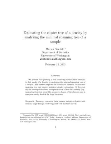
Measuring agreement between partitions. Let P1 and P2 be twopartitions of a set of n objects. The partitions define a contingency table:let nij be the number of objects that belong to subset i of partition P1 andto subset j of partition P2 . We measure the agreement between P1 and P2by the adjusted Rand index (Hubert and Arabie 1985) defined as nij R ij12 ni·i2 ni· n·j n / 2i 2j22 n·j ni· n·j n j 2i2j2/.2 Here ni· j nij , and n·j is defined analogously.The adjusted Rand index has a maximum value of 1 which is achievedwhen the two partitions are identical up to re-numbering of the subsets. Ithas expected value 0 under random assignment of the objects to the subsetsof P1 and P2 that leave the marginals ni· and n·j fixed.Choosing a partition size. Choosing a partition size is a difficult issue,especially for nonparametric clustering methods, for which there is as yetno automatic method, and subjective judgment is required. To eliminatethe subjective element from the comparisons, we decompose the clusteringproblem into two subproblems: (a) determining the number of groups, and(b) finding the groups, given their number. We compare the performance onsubproblem (b), using two different rules for setting the number of groups.First, we have each method produce the true number of groups. Second, wegenerate a range of partitions of different sizes, calculate the adjusted Randindex for each of them, and then report the maximum value of the indexachieved by the method and the corresponding partition size.5.2Nonlinear clusters — BullseyeThe data used in this example are shown in Figure 4(a). There are 500observations uniformly distributed over the center of the bullseye and thering. Figure 4(b) shows the 2-partition generated by runt pruning of theMST. Figures 4(c),. . . , 4(e) show the 2-partitions generated by single, average, and complete linkage, respectively. Figure 4(f) shows the 2-partitiongenerated by fitting Gaussian mixtures. We used the software described inFraley and Raftery (1999). The Gaussians were constrained to have equalspherical covariance matrices.12
Figure 4: (a) Observations; (b). . . (f) 2-partitions found by (b) runt analysis,(c) single linkage, (d) average linkage, (e) complete linkage, (f) model-basedclustering.Runt pruning correctly identifies the two clusters, as does single linkageclustering. Single linkage performs well in this example because the Hausdorffdistance between the groups is large compared to the typical nearest neighbordistance. The other methods all fail in similar ways. This result is notsurprising, because they are all designed to find roughly convex clusters.5.3Gaussian clusters — SimplexThe data in this example consist of spherical Gaussian clusters with commonstandard deviation σ 0.25, centered at the vertices of the unit simplex inp 1 dimensions.The first example is for p 3, with cluster sizes 100, 200, and 300,13
respectively. The runt sizes of the MST are, in descending order, 194, 94, 29,29, 20, 20, 20, 19, 15, 15, 12, 11, 11, 10, 10, . . . . There is a big gap after 94,suggesting the presence of three modes.Figure 5(a) shows the cluster tree, with the root node selected. Panel (b)shows the descendents of the root node. In panel (c) we have selected theright daughter of the root node. Panel (d) shows its descendents.Figure 5: (a) Cluster tree for tri-modal Gaussian data with root node selected; (b) left and right descendents of root node; (c) cluster tree with rightdaughter of root node selected; (d) left and right descendents.In this simple example, average and complete linkage, runt analysis, andmodel-based clustering all do an excellent job of finding the groups whenasked to produce a 3-partition. The exception is single linkage clustering.Breaking the two longest edges of the MST results in two clusters of size 1and one cluster containing the rest of the data.14
SLALCLRPMC-EIMC-VI0.0 (0.03) 0.92 (0.01) 0.92 (0.04) 0.82 (0.05) 0.93 (0.02) 0.92 (0.01)0.0 (0.08) 0.92 (0.01) 0.92 (0.02) 0.90 (0.03) 0.93 (0.02) 0.92 (0.01)1677877Table 1: Comparison of single, average, and complete linkage, runt pruning,and two versions of model-based clustering for seven-dimensional simplexdata. First row: adjusted Rand index if methods are made to generate sevenclusters; second row: adjusted Rand index for optimal partition size; thirdrow: optimal partition size. Numbers in parentheses are standard errors.We next consider dimensionality p 7, with cluster sizes 50, 60, . . . , 110.The runt sizes are 80, 73, 60, 38, 35, 26, 14, 10, 9, 9, 8, 7, 6, 6, 6.Table 1 summarizes the performance of single, average, and complete linkage, runt analysis, and two versions of model-based clustering, fitting spherical Gaussians with equal variance and fitting spherical Gaussians with unequal variances. The first row of the table contains the values of the adjustedRand index when the methods are asked to construct a 7-partition. The second row contains the optimal values of the index (optimized over partitionsize). Numbers in parentheses are standard errors obtained by half-sampling(Shao and Tu 1995, Section 5.2.2). All methods except single linkage clustering perform well, although runt pruning appears to fall off a little.5.4Olive oil dataThe data for this example consist of measurements of eight chemical concentrations on 572 samples of olive oil. The samples come from three differentregions of Italy. The regions are further partitioned into nine areas: areasA1. . . A4 belong to region R1, areas A5 and A6 belong to region R2, andareas A7. . . A9 belong to region R3. We did not scale or sphere the data, because the variables are already on the same scale. The largest runt sizes were168, 97, 59, 51, 42, 42, 33, 13, 13, 12, 11, 11, 11, 10, 10,. . . . The gap after33 suggests the presence of eight modes. We thus chose runt size threshold33 in the construction of the cluster tree. (The picture often is not as clear.)Figure 6 shows the cluster tree. We have labeled each leaf with the predominant area for the olive oil samples falling into this leaf. Table 2 shows15
Figure 6: Cluster tree for olive oil data. Nodes have been labeled withpredominant area.the distribution of areas over clusters. Table 3 summarizes the performanceof clustering methods for the olive oil date. Runt pruning with threshold 33(eight clusters) gives an adjusted Rand index of 0.57. Again, single linkageis the lone outlier.The split represented by the root node separates region R3 from regionsR1 and R2. The left daughter separates region R1 from region R2. Themethod erroneously splits area A3 into two clusters and was not successfulin identifying areas A1 and A4. This raises two questions: (a) do the oliveoils from area A3 really have a bimodal density, and (b) does the densityreally have modes corresponding to areas A1 and A4?The first question is at least partly answered by Figure 7. Panel (a) showsthe cluster tree. We have selected the node N that has partitioned area A3.Panel (b) shows a rootogram (histogram with the roots of the cell countsplotted on the vertical axis) of the cluster represented by N, projected ontothe Fisher discriminant direction calculated to separate the daughter clusters.(The idea for this diagnostic plot comes from Gnanadesikan, Kettenring, andLandwehr (1982). The Fisher discriminant direction maximizes the ratioof between-cluster variance to within-cluster variance of the projected data(Mardia, Kent, and Bibby 1979, Section 11.5). In that sense it is the direction16
1 2A1 0 1A2 0 51A3 90 11A4 5 13A5 0 0A6 0 0A7 0 3A8 0 2A9 0 03 4 5 6 7 80 0 0 17 0 71 0 0 4 0 0103 1 0 0 1 04 0 0 14 0 00 64 1 0 0 00 0 33 0 0 00 0 0 43 0 40 0 0 2 45 10 0 0 0 0 51Table 2: Olive oil data: cluster number (horizontal axis) tabulated againstarea (vertical axis).that best reveals separation between clusters.) The rootogram does not lookbimodal. While this does not conclusively show that there is only one mode— there might be two modal regions with nonlinear shapes, so that theseparation does not manifest itself in the projection — it is an indication,and we might want to prune the tree by removing the daughters. In contrast,the rootogram in panel (d) where we have selected the node separating areaA2 from area A3, shows clear bimodality. Note that this diagnostic can beused in practical problems because it does not require knowing the true labelsof the observations.To answer the question whether areas A1 and A4 really are separated fromareas A2 and A3 and correspond to modes of the density, we project theobservations from the four areas onto the first two discriminant coordinates(Mardia, Kent, and Bibby 1979, Section 12.5). Figure 8 shows that whileareas A2 (open circle) and A3 (filled circle) form fairly obvious groups, thisis not true for areas A1 (triangle) and A4 (cross). Again, finding this is notstrictly conclusive because we are seeing only a two-dimensional projectionof the eight-dimensional data but it is a good indication. Note that thisapproach is not an “operational” diagnostic, because in practice the truelabels of the observations would be unknown. We use it here merely to helpevaluate the performance of our method.17
Figure 7: Diagnostic plots. Panel (a): cluster tree with node splitting area A3selected; (b) projection of data in node on the Fisher discriminant directionseparating daughters; (c) cluster tree with node separating area A3 from areaA2 selected; (d) projection of data on the Fisher discriminant direction.5.5Handwritten digit dataThe data for this example are 2,000 16 16 grey level images of handwrittendigits; the data therefore are of dimensionality 256. (The data were previously used to evaluate machine learning algorithms). The runt sizes are 288,283, 90, 84, 74, 47, 37, 35, 22, 21, 21, 19, 19, 18, 13, 12, 12,. . . . The gapafter 35 (vaguely) suggests presence of nine groups.Table 4 summarizes the performance of various clustering methods on thehandwritten digit data. The clear winners are model-based clustering withidentical, spherical covariance matrices, and runt pruning. Runt pruningwith threshold 35 (nine clusters) gives an adjusted Rand index of 0.64. Thepoor performance of average linkage is surprising.18
Figure 8: Projection of areas A1 (triangle), A2 (open circle), A3 (filled circle),and A4 (cross) on the plane spanned by first two discriminant coordinates.6RemarksWe addre
Figure 2: Density and corresponding tree of high density clusters. ters at a given density level λ chosen by the user. The idea is to first compute a kernel density estimate ˆp (Silverman 1986, Chapter 4) and set aside all ob- servations with ˆp(xi) λ, i.e., all observations not in the level set L(λ;ˆp). If the population de