Transcription
Chapter16Cluster AnalysisIdentifying groups of individuals or objects that are similar to each other but differentfrom individuals in other groups can be intellectually satisfying, profitable, orsometimes both. Using your customer base, you may be able to form clusters ofcustomers who have similar buying habits or demographics. You can take advantageof these similarities to target offers to subgroups that are most likely to be receptiveto them. Based on scores on psychological inventories, you can cluster patients intosubgroups that have similar response patterns. This may help you in targetingappropriate treatment and studying typologies of diseases. By analyzing the mineralcontents of excavated materials, you can study their origins and spread.Tip: Although both cluster analysis and discriminant analysis classify objects (orcases) into categories, discriminant analysis requires you to know group membershipfor the cases used to derive the classification rule. The goal of cluster analysis is toidentify the actual groups. For example, if you are interested in distinguishingbetween several disease groups using discriminant analysis, cases with knowndiagnoses must be available. Based on these cases, you derive a rule for classifyingundiagnosed patients. In cluster analysis, you don’t know who or what belongs inwhich group. You often don’t even know the number of groups.Examples You need to identify people with similar patterns of past purchases so that you cantailor your marketing strategies.361
362Chapter 16 You’ve been assigned to group television shows into homogeneous categoriesbased on viewer characteristics. This can be used for market segmentation. You want to cluster skulls excavated from archaeological digs into the civilizationsfrom which they originated. Various measurements of the skulls are available. You’re trying to examine patients with a diagnosis of depression to determine ifdistinct subgroups can be identified, based on a symptom checklist and results frompsychological tests.In a NutshellYou start out with a number of cases and want to subdivide them into homogeneousgroups. First, you choose the variables on which you want the groups to be similar.Next, you must decide whether to standardize the variables in some way so that theyall contribute equally to the distance or similarity between cases. Finally, you have todecide which clustering procedure to use, based on the number of cases and types ofvariables that you want to use for forming clusters.For hierarchical clustering, you choose a statistic that quantifies how far apart (orsimilar) two cases are. Then you select a method for forming the groups. Because youcan have as many clusters as you do cases (not a useful solution!), your last step is todetermine how many clusters you need to represent your data. You do this by lookingat how similar clusters are when you create additional clusters or collapse existing ones.In k-means clustering, you select the number of clusters you want. The algorithmiteratively estimates the cluster means and assigns each case to the cluster for which itsdistance to the cluster mean is the smallest.In two-step clustering, to make large problems tractable, in the first step, cases areassigned to “preclusters.” In the second step, the preclusters are clustered using thehierarchical clustering algorithm. You can specify the number of clusters you want orlet the algorithm decide based on preselected criteria.IntroductionThe term cluster analysis does not identify a particular statistical method or model, asdo discriminant analysis, factor analysis, and regression. You often don’t have to makeany assumptions about the underlying distribution of the data. Using cluster analysis,you can also form groups of related variables, similar to what you do in factor analysis.There are numerous ways you can sort cases into groups. The choice of a method
363Cluster Analy sisdepends on, among other things, the size of the data file. Methods commonly used forsmall data sets are impractical for data files with thousands of cases.SPSS has three different procedures that can be used to cluster data: hierarchicalcluster analysis, k-means cluster, and two-step cluster. They are all described in thischapter. If you have a large data file (even 1,000 cases is large for clustering) or amixture of continuous and categorical variables, you should use the SPSS two-stepprocedure. If you have a small data set and want to easily examine solutions withincreasing numbers of clusters, you may want to use hierarchical clustering. If youknow how many clusters you want and you have a moderately sized data set, you canuse k-means clustering.You’ll cluster three different sets of data using the three SPSS procedures. You’lluse a hierarchical algorithm to cluster figure-skating judges in the 2002 OlympicGames. You’ll use k-means clustering to study the metal composition of Romanpottery. Finally, you’ll cluster the participants in the 2002 General Social Survey,using a two-stage clustering algorithm. You’ll find homogenous clusters based oneducation, age, income, gender, and region of the country. You’ll see how Internet useand television viewing varies across the clusters.Hierarchical ClusteringThere are numerous ways in which clusters can be formed. Hierarchical clustering isone of the most straightforward methods. It can be either agglomerative or divisive.Agglomerative hierarchical clustering begins with every case being a cluster untoitself. At successive steps, similar clusters are merged. The algorithm ends witheverybody in one jolly, but useless, cluster. Divisive clustering starts with everybody inone cluster and ends up with everyone in individual clusters. Obviously, neither thefirst step nor the last step is a worthwhile solution with either method.In agglomerative clustering, once a cluster is formed, it cannot be split; it can onlybe combined with other clusters. Agglomerative hierarchical clustering doesn’t letcases separate from clusters that they’ve joined. Once in a cluster, always in that cluster.To form clusters using a hierarchical cluster analysis, you must select: A criterion for determining similarity or distance between cases A criterion for determining which clusters are merged at successive steps The number of clusters you need to represent your data
364Chapter 16Tip: There is no right or wrong answer as to how many clusters you need. It dependson what you’re going to do with them. To find a good cluster solution, you must lookat the characteristics of the clusters at successive steps and decide when you have aninterpretable solution or a solution that has a reasonable number of fairlyhomogeneous clusters.Figure-Skating Judges: The ExampleAs an example of agglomerative hierarchical clustering, you’ll look at the judging ofpairs figure skating in the 2002 Olympics. Each of nine judges gave each of 20 pairs ofskaters four scores: technical merit and artistry for both the short program and the longprogram. You’ll see which groups of judges assigned similar scores. To make theexample more interesting, only the scores of the top four pairs are included. That’swhere the Olympic scoring controversies were centered. (The actual scores are onlyone part of an incredibly complex, and not entirely objective, procedure for assigningmedals to figure skaters and ice dancers.)*Tip: Consider carefully the variables you will use for establishing clusters. If you don’tinclude variables that are important, your clusters may not be useful. For example, ifyou are clustering schools and don’t include information on the number of students andfaculty at each school, size will not be used for establishing clusters.How Alike (or Different) Are the Cases?Because the goal of this cluster analysis is to form similar groups of figure-skatingjudges, you have to decide on the criterion to be used for measuring similarity ordistance. Distance is a measure of how far apart two objects are, while similaritymeasures how similar two objects are. For cases that are alike, distance measures aresmall and similarity measures are large. There are many different definitions ofdistance and similarity. Some, like the Euclidean distance, are suitable for onlycontinuous variables, while others are suitable for only categorical variables. There arealso many specialized measures for binary variables. See the Help system for adescription of the more than 30 distance and similarity measures available in SPSS.* I wish to thank Professor John Hartigan of Yale University for extracting the data fromwww.nbcolympics.com and making it available as a data file.
365Cluster Analy sisWarning: The computation for the selected distance measure is based on all of thevariables you select. If you have a mixture of nominal and continuous variables, youmust use the two-step cluster procedure because none of the distance measures inhierarchical clustering or k-means are suitable for use with both types of variables.To see how a simple distance measure is computed, consider the data in Figure 16-1.The table shows the ratings of the French and Canadian judges for the Russian pairsfigure skating team of Berezhnaya and Sikhardulidze.Figure 16-1Distances for two judges for one pairLong ProgramShort ProgramJudgeTechnical MeritArtistryTechnical ou see that, for the long program, there is a 0.1 point difference in technical meritscores and a 0.1 difference in artistry scores between the French judge and theCanadian judge. For the short program, they assigned the same scores to the pair. Thisinformation can be combined into a single index or distance measure in many differentways. One frequently used measure is the squared Euclidean distance, which is the sumof the squared differences over all of the variables. In this example, the squaredEuclidean distance is 0.02. The squared Euclidean distance suffers from thedisadvantage that it depends on the units of measurement for the variables.Standardizing the VariablesIf variables are measured on different scales, variables with large values contributemore to the distance measure than variables with small values. In this example, bothvariables are measured on the same scale, so that’s not much of a problem, assumingthe judges use the scales similarly. But if you were looking at the distance between twopeople based on their IQs and incomes in dollars, you would probably find that thedifferences in incomes would dominate any distance measures. (A difference of only 100 when squared becomes 10,000, while a difference of 30 IQ points would be only900. I’d go for the IQ points over the dollars!) Variables that are measured in largenumbers will contribute to the distance more than variables recorded in smallernumbers.
366Chapter 16Tip: In the hierarchical clustering procedure in SPSS, you can standardize variables indifferent ways. You can compute standardized scores or divide by just the standarddeviation, range, mean, or maximum. This results in all variables contributing moreequally to the distance measurement. That’s not necessarily always the best strategy,since variability of a measure can provide useful information.Proximity MatrixTo get the squared Euclidean distance between each pair of judges, you square thedifferences in the four scores that they assigned to each of the four top-rated pairs. Youhave 16 scores for each judge. These distances are shown in Figure 16-2, the proximitymatrix. All of the entries on the diagonal are 0, since a judge does not differ fromherself or himself. The smallest difference between two judges is 0.02, the distancebetween the French and Russian judges. (Look for the smallest off-diagonal entry inFigure 16-2.) The largest distance, 0.25, occurs between the Japanese and Canadianjudges. The distance matrix is symmetric, since the distance between the Japanese andRussian judges is identical to the distance between the Russian and Japanese judges.Figure 16-2Proximity matrix between judgesTip: In Figure 16-2, the squared Euclidean distance between the French and Canadianjudge is computed for all four pairs. That’s why the number differs from that computedfor just the single Russian pair.
367Cluster Analy sisHow Should Clusters Be Combined?Agglomerative hierarchical clustering starts with each case (in this example, eachjudge) being a cluster. At the next step, the two judges who have the smallest value forthe distance measure (or largest value if you are using similarities) are joined into asingle cluster. At the second step, either a third case is added to the cluster that alreadycontains two cases or two other cases are merged into a new cluster. At every step,either individual cases are added to existing clusters, two individuals are combined, ortwo existing clusters are combined.When you have only one case in a cluster, the smallest distance between cases intwo clusters is unambiguous. It’s the distance or similarity measure you selected forthe proximity matrix. Once you start forming clusters with more than one case, youneed to define a distance between pairs of clusters. For example, if cluster A has cases1 and 4, and cluster B has cases 5, 6, and 7, you need a measure of how different orsimilar the two clusters are.There are many ways to define the distance between two clusters with more than onecase in a cluster. For example, you can average the distances between all pairs of casesformed by taking one member from each of the two clusters. Or you can take the largestor smallest distance between two cases that are in different clusters. Different methodsfor computing the distance between clusters are available and may well result indifferent solutions. The methods available in SPSS hierarchical clustering aredescribed in “Distance between Cluster Pairs” on p. 372.Summarizing the Steps: The Icicle PlotFrom Figure 16-3, you can see what’s happening at each step of the cluster analysiswhen average linkage between groups is used to link the clusters. The figure is calledan icicle plot because the columns of X’s look (supposedly) like icicles hanging fromeaves. Each column represents one of the objects you’re clustering. Each row shows acluster solution with different numbers of clusters. You read the figure from the bottomup. The last row (that isn’t shown) is the first step of the analysis. Each of the judges isa cluster unto himself or herself. The number of clusters at that point is 9. The eightcluster solution arises when the Russian and French judges are joined into a cluster.(Remember they had the smallest distance of all pairs.) The seven-cluster solutionresults from the merging of the German and Canadian judges into a cluster. The sixcluster solution is the result of combining the Japanese and U.S. judges. For the onecluster solution, all of the cases are combined into a single cluster.
368Chapter 16Warning: When pairs of cases are tied for the smallest distance, an arbitrary selectionis made. You might get a different cluster solution if your cases are sorted differently.That doesn’t really matter, since there is no right or wrong answer to a cluster analysis.Many groupings are equally plausible.Figure 16-3Vertical icicle plotTip: If you have a large number of cases to cluster, you can make an icicle plot in whichthe cases are the rows. Specify Horizontal on the Cluster Plots dialog box.Who’s in What Cluster?You can get a table that shows the cases in each cluster for any number of clusters.Figure 16-4 shows the judges in the three-, four-, and five-cluster solutions.Figure 16-4Cluster membership
369Cluster Analy sisTip: To see how clusters differ on the variables used to create them, save the clustermembership number using the Save command and then use the Means procedure,specifying the variables used to form the clusters as the dependent variables and thecluster number as the grouping variable.Tracking the Combinations: The Agglomeration ScheduleFrom the icicle plot, you can’t tell how small the distance measure is as additional casesare merged into clusters. For that, you have to look at the agglomeration schedule inFigure 16-5. In the column labeled Coefficients, you see the value of the distance (orsimilarity) statistic used to form the cluster. From these numbers, you get an idea ofhow unlike the clusters being combined are. If you are using dissimilarity measures,small coefficients tell you that fairly homogenous clusters are being attached to eachother. Large coefficients tell you that you’re combining dissimilar clusters. If you’reusing similarity measures, the opposite is true: large values are good, while smallvalues are bad.The actual value shown depends on the clustering method and the distance measureyou’re using. You can use these coefficients to help you decide how many clusters youneed to represent the data. You want to stop cluster formation when the increase (fordistance measures) or decrease (for similarity measures) in the Coefficients columnbetween two adjacent steps is large. In this example, you may want to stop at the threecluster solution, after stage 6. Here, as you can confirm from Figure 16-4, the Canadianand German judges are in cluster 1; the Chinese, French, Polish, Russian, andUkrainian judges are in cluster 2; and the Japanese and U.S. judges are in cluster 3. Ifyou go on to combine two of these three clusters in stage 7, the distance coefficientacross the last combination jumps from 0. 093 to 0.165.
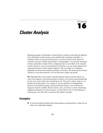
370Chapter 16Figure 16-5Agglomeration scheduleThe agglomeration schedule starts off using the case numbers that are displayed on theicicle plot. Once cases are added to clusters, the cluster number is always the lowest ofthe case numbers in the cluster. A cluster formed by merging cases 3 and 4 wouldforever be known as cluster 3, unless it happened to merge with cluster 1 or 2.The columns labeled Stage Cluster First Appears tell you the step at which each ofthe two clusters that are being joined first appear. For example, at stage 4 when cluster3 and cluster 6 are combined, you’re told that cluster 3 was first formed at stage 1 andcluster 6 is a single case and that the resulting cluster (known as 3) will see action againat stage 5. For a small data set, you’re much better off looking at the icicle plot thantrying to follow the step-by-step clustering summarized in the agglomeration schedule.Tip: In most situations, all you want to look at in the agglomeration schedule is thecoefficient at which clusters are combined. Look at the icicle plot to see what’s going on.Plotting Cluster Distances: The DendrogramIf you want a visual representation of the distance at which clusters are combined, youcan look at a display called the dendrogram, shown in Figure 16-6. The dendrogram isread from left to right. Vertical lines show joined clusters. The position of the line onthe scale indicates the distance at which clusters are joined. The observed distances arerescaled to fall into the range of 1 to 25, so you don’t see the actual distances; however,the ratio of the rescaled distances within the dendrogram is the same as the ratio of theoriginal distances.The first vertical line, corresponding to the smallest rescaled distance, is for theFrench and Russian alliance. The next vertical line is at the same distances for three
371Cluster Analy sismerges. You see from Figure 16-5 that stages 2, 3, and 4 have the same coefficients.What you see in this plot is what you already know from the agglomeration schedule.In the last two steps, fairly dissimilar clusters are combined.Figure 16-6The dendrogramDendrogram using Average Linkage (Between Groups)Rescaled Distance Cluster CombineC A S GermanyNum0510152025 --------- --------- --------- --------- --------- 376285914« ««««««««««««« « ²««« ««««««««««««««« ²« ««««««««««««««««««« ²««««««««««««««««««««« «««««««««««««
Cluster Analysis depends on, among other things, the size of the data file. Methods commonly used for small data sets are impractical for data files with thousands of cases. SPSS has three different procedures that can be used to cluster data: hierarchical cluster analysis, k-means cluster, and two-step cluster. They are all described in thisFile Size: 1MB