Transcription
28TH INTERNATIONAL CONGRESS OF THE AERONAUTICAL SCIENCESTURBOJET ANALYTICAL MODEL DEVELOPMENTAND VALIDATIONS. Chiesa*, G. Medici*, M. Balbo***Politecnico di Torino, **Alenia Aermacchisergio.chiesa@polito.it; giovanni.medici@polito.it; massimo.balbo@alenia.itKeywords: Turbojet; Steady State; Transient; Thrust Vectoring; CFDAbstractThis paper describes the modeling andvalidation procedure of a single shaft turbojetengine. The model aim is to provide detailedpredictions of the flow’s properties at nozzleoutlet. Those predictions will be used to designa thrust vectoring system for the engine, and theflight dynamics control laws of the aircraft.The first phase of the analysis explains thedesign and development a more detailed enginedeck. The engine to model is a single shaftturbojet. The software developed calculates theturbojet performances in steady state; boundaryconditions of the turbojet may be modifiedaccording to the engine-operating envelope.During the second phase of the analysis,the transient model was developed. Droppingthe work compatibility equation, andintroducing the angular acceleration andinertial moments allow to model the engine vs.time behavior.By using the data calculated through thesteady state and transient 1-D models, the CFDmodel could be properly designed. The modeldefines the flow field going from the turbine’soutlet through the nozzle to the turbojet plumedownstream. In this way the estimation of theforces and moments acting on the thrustvectoring vanes can be calculated. The threemodels were validated using test bench data,synthetic data (previous steady state enginedecks) and flight test data.1General IntroductionSince 2010 Alenia Aermacchi (joined withPolitecnico di Torino) is offering an IndustrialPh.D scholarship program, in order to work onsome of the company’s research fields (i.e. [4],[6], [11]). In particular in order to study a thrustvectoring Unmanned Aerial Vehicle (UAV)application, an initial survey on a turbojetturbine and nozzle performances wasconducted. The turbojet engine studied pushesthe Alenia Aermacchi’s Sky-X UAV, atechnological demonstrator (Fig. 1). In literaturethere are many examples of turbojet steady statemodeling methods [7], and [10], some of themhave been developed in order to calculatetransients too [14]. The models presented in thispaper are based on such methods; to validatethem real turbojet engine data (data calculatedthrough a computer deck software, test benchdata, and flight data) was used.Fig. 1. Sky-X UAVThis section introduces the research; in thesecond part of the paper the 1-D, steady stateand transient model is described, while the thirdsection contains the CFD model. The latter usesextensively the results of 1-D models in order todefine the boundary conditions. In the last partresults are reported and commented.21-D ModelsIn the first phase of the development a steadystate analytical model was designed. The modelwas built to obtain a more detailed engine deck.1
S. CHIESA, G. MEDICI, M. BALBOThe engine to model is configured with:single shaft, three stage axial compressor (fixedgeometry, without any Inlet Guide Vanes IGV),single stage turbine, annular combustionchamber, fixed nozzle, pure turbojet. The simpleconfiguration of the gas turbine, allows tomodel several components maps (that areunknown) by using an analytical deck [10], and[13]. Since many components lack of detailedinformation few simplifications were introducedin the model.Steady State Model LayoutThe software developed, based on Matlab,models a steady state, variable RPM andboundary conditions turbojet. The programcalculates engine performances (e.g. mass flowrate, temperature, pressure.), in every stage. Itis a 1-D (one dimensional) model, meaning thatthe engine was cut stage by stage in thelongitudinal plane (Fig. 4), and every property iscalculated as a mean value in each stage.Matlab programming language is used dueto its fast implementation yet powerful routinesand matrix management tools. During thecalculation the isentropic coefficient, specificheat coefficient, and combustion chamberTemperature rise values depend uponTemperature and fuel/air ratio. This choiceaffects the algorithm process flow (introducesfew iterations), but the overall CPU requirementof the algorithm is modest, and allows real-timecalculation. The model can be controlledthrough a GUI (Fig. 2), that contains theboundary conditions parameters to set: altitude,and temperature relative to ISA standards, Mach( Ma ), Fuel lower heating value ( H u ), extractedpower ( Pe ), percent of bleed air flow ( β% ), andair intake isentropic efficiency ( ηin ).Once every parameter is set, a routineverifies that the analysis point requested liesinside the engine envelope (Fig. 3). Thesoftware is modular, and its boundary conditioninitialization procedure allows it to be veryflexible and customizable. It is possible, forexample, to modify the operating envelope, byintroducing the new conditions in a separate textfile. Other engine internal parameters, such asFig. 2. Steady State Model GUIEngine Operating Flight Envelope10.83Altitude/Altituderef [ ]2.1efficiencies, and iteration parameters, can beadjusted in a separate input file as well.0.670.50.33Nidle min XXXXX RPM0.17Nidle min XXXXX RPMNidle min XXXXX RPM000.10.20.30.40.5Mach0.60.70.80.91Fig. 3. Engine Operating Flight EnvelopeFig. 4. Turbojet stage numbering2.2Steady State Model AlgorithmOff-design equilibrium running calculation isbased on satisfying the flow and workcompatibility between the components [12]:(a) The user chooses the boundary conditions(altitude, Mach, and variation from the ISA2
TURBOJET ANALYTICAL MODEL DEVELOPMENT ANDVALIDATIONdayΔTISA ).Airintake'sinletpressure ratio, the pressure ratio of the gasgenerator turbine can be found. Thisapproximation effectively fixes the valuestotaltemperature ( T ) is calculated through (1),00where ( γ 0 ) is the isentropic coefficient inair intake's inlet section, ( Ma ) is the Machnumber at air intake inlet section and ( T10 )is the total temperature at air intake outletsection (the flow starting at infinite andgoing through the air intake does notexchange heat and work thus the totaltemperature remains constant): γ 1 T00 T10 Ta 1 0Ma 2 2(1)of corrected turbine mass flow,and turbine temperature ratio,γ0(2)(b) By picking a compressor constant-speedline on the compressor characteristic,p0compressor pressure ratio 2 0 , correctedp1m T10, and efficiency ( ηc ) ofp10the compressor can be defined.(c) The compressor total temperature ratio canbe calculated through the (3):airflow 0 γγ 1 T p2 ΔT10, 2 0 1 ηc p1 01(3)(d) Nozzle map can be simplified as a singleline characteristic map, and since theturbine characteristic does not changeconsiderably with the RPM, a single linecharacteristic map can be used for theturbine too.(e) Afore mentioned simplification allows aneasier calculation of the complete turbojetcycle. In particular for a given compressorp30,0ΔT3,4.T30(f) In this way a single iteration is sufficient tofind the equilibrium running point on eachcompressor constant speed line.(g) The compressor and turbine sides are linkedby equations (4) and (5):There are total pressure losses, due to airintake's isentropic efficiency ( ηin ), in thestages 0-1. Total temperature and intakeefficiency gives air intake’s outlet totalpressure ( p10 ) (2): T 0 γ 0 1p10 pa 1 ηin 1 1 Ta m T300c p,12ΔT1,20 T10ΔT3.4 0 0 0T3T1 T3 ηmech c p.34(4)m T30 m T10 p10 p20 T30 m3 0 0 p30p10p2 p3 T10 m1(5)(h) The iteration matches the0ΔT3,4value.T30By estimating compressor and turbine’sequilibrium points, every property of eachturbojet’s stage can be calculated. The tooliterates on each isentropic coefficient and on theconstant pressure heat coefficients ( c p ).The original compressor map shows onlyfew constant speed lines, a compressor mapscale routine was developed in order to refinethe compressor characteristic map. Thanks tothe lookup table the plot of a property withrespect to the RPM results smoother.During the development of this tool severalturbojet’s unknowns had to be estimated. Thegeneral map of a component (compressor,turbine, nozzle) was usually available, or couldbe calculated, but the components’ efficiencieshad to be estimated. By choosing accordinglythe components efficiencies, using referenceengine examples, a close match with theexperimental turbojet data is achieved.2.3Steady State Model OutputThe steady state model allows calculating 56parameters on five stages of the turbojet, whilethe original deck could only calculate 123
S. CHIESA, G. MEDICI, M. BALBOTable 1. Sea level standard and cruise boundaryconditionsHu42800 [kJ/kg]Pe0.1 [kW]hSLS0 [km]0 [-]Ma2.4ηin0.98 [-]ΔTISA0 [K]hCruise5 [km]0.3 [-]MaTransient ModelDuring the second phase of the analysis, thetransient model was developed. The transientmodel calculates Engine’s dynamics (propertiesvariation vs. time), by dropping the workcompatibility equation, and introducing theangular acceleration and inertial moments. Thetransient model uses the same Matlab functiondeveloped for the steady state to calculate stageby stage properties, while the time dependingdynamics are calculated using Simulink. Themodel is 1-D and does not include anyinformation on the wall temperatures (no walltemperature inertia has been modeled).Deck, Steady State Model Comparison, Corrected Thrust1.18h0 m0 t0 deck d1.060.95Steady State Modelh0 m0 t0 deck jFc/Fcref [ PMc/RPMref [ ]0.941.011.08Fig. 5. Sea Level Standard Corrected Thrust.Deck, Steady State Model Comparison, Corrected Airflow1.060.980.910.83mc/mcref [ ]parameters. The source code can be accessedand adjusted as desired (in order to adapt it to adifferent engine). The model provides variousplot tools that allows creating comparisonbetween different simulations. For example it ispossible to check the way the turbojet cyclechanges due to the variation of air intakeefficiency, Mach, or altitude.Fig. 5, and Fig. 6, depict a comparisonbetween two versions of the original deck andthe actual steady state model. The figures showtwo of the most important turbojet engine’sproperties: thrust, and airflow. Table 1summarizes the boundary conditions used in thecomparison (Sea Level Standard, SLS). Resultsare presented with respect to the reference valueof each property. The trend of the steady statemodel matches the one of the original decks.The original deck used text files as inputand output. This kind of format forces datamanagement to be performed only manually(frustrating) or by a text file parsing routine(that could give rise to errors due to particulartext formatting of the output file). In order toovercome this flaw the developed tool outputsData that can be saved and accessed.0.76h0 m0 t0 deck d0.68Steady State Modelh0 m0 t0 deck j0.60.530.450.610.670.740.810.88RPMc/RPMref [ ]0.941.011.08Fig. 6. Sea Level Standard Corrected airflow.2.5Transient Model AlgorithmIn the transient model while the flowcompatibility holds, work compatibility betweencompressor and turbine drops. The net–workbetween the two components induces theturbojet spool to accelerate or decelerate. TheNewton’s Second Law of Motion can be used torelate compressor’s acceleration and the excessof torque ( ΔG ):ΔG J ω (6)In equation (6) the angular acceleration ofthe rotor ( ω ) is known, the polar moment ofinertia ( J ) was estimated using a dry crank testdata. Initially the turbojet engine wasaccelerated to a known RPM speed. The torque4
TURBOJET ANALYTICAL MODEL DEVELOPMENT ANDVALIDATION( Cknown ) was then removed and leaving theengine’s spool free to rotate. By knowing thetime the engine takes to stop, its polar momentof inertia was estimated (7).Cknown J ω J RPM drycrankdω J dtttostop(7)The torque excess can be writtenconsidering turbine and compressor loads (8):ΔG Gt Gc(8)Since turbine and compressor’s power canbe written as (9), and (10):()Pt ηm m a m f c p,34 ΔT3,40(9)Pc m a c p,12 ΔT1,20(10)exceeds 98%, and the engine is accelerating, theECU dumps the fuel flow ramp. When theExhaust Gas Temperature (EGT), or itsderivative, exceeds a threshold the ECU cuts10% of the fuel flow.2.6Transient Model GUIThe layout of the model differs slightly from thesteady state one, as it must provide the featureof changing the boundary conditions during thesimulation (Fig. 7 and Fig. 8). The Simulinkenvironment is particularly effective for thesimulation of controllers and logics, such asEngine Control Unit [1], [5], [8], and [9].The torque excess can be calculated byusing the (11):ΔG ()0ηmech m a m f c p,34 ΔT 34m a c p,12 ΔT120 2π N2π N (11)Where ( c p,12 ) and ( c p,34 ) are the constantpressure heat coefficients related to thecompressor and the turbine; while airflow massand fuel flow mass are ( m a ) and ( m f ). Now byknowing the polar moment of inertia and thesimulation's time step is possible to calculate thetransient running points of the turbojet. Due tothe simple geometry of the engine, and relativeslow dynamics (65% 100% slam takes 6 – 8seconds), the volume inside each componentcan be assumed constant, so that pressure andtemperature change instantly and massconservation holds.The basic engines dynamics are defined bythe equations described before, but the realturbojet contains an Engine Control Unit (ECU),that manages fuel flow depending on thermal ormechanical constraints. By analyzing theengines time histories an elementary ECU wasmodeled in Simulink. The ECU block changesthe fuel flow according to the RPM. When itFig. 7. Transient Model Compressor Map.Single Shaft Turbojet Transient ModelD0ClockONC0EGTFuel FlowAEGT PatchDFromHOFFDelta TdeltaISAh Sim [km]BONMachBENVMach SimOFFAENVIRONMENT SpeedRPMRPMhThrottle Display K throttleFADECTransientGiovanni Medici 2012Fig. 8. Transient Model GUIDuring the simula
them real turbojet engine data (data calculated through a computer deck software, test bench data, and flight data) was used. Fig. 1. Sky-X UAV This section introduces the research; in the second part of the paper the 1-D, steady state and transient model is described, while the third section contains the CFD model. The latter uses extensively the results of 1-D models in order to define the .