Transcription
Lecture NotesFundamentals of Big DataAnalyticsProf. Dr. Rudolf MatharRheinisch-Westfälische Technische Hochschule AachenLehrstuhl für Theoretische InformationstechnikKopernikusstraße 1652074 AachenVersion from January 18, 2019
Contents1 Introduction1.1 MapReduce and Hadoop . . . . . . . . . . . . . . . . . . . . . . . . . . . . .562 Prerequisites from Matrix Algebra92.1 Projection and Isometry . . . . . . . . . . . . . . . . . . . . . . . . . . . . . 133 Multivariate Distributions and Moments3.1 Random Vectors . . . . . . . . . . .3.2 Expectation and Covariance . . . . .3.3 Conditional Distribution . . . . . . .3.4 Maximum Likelihood Estimation . .17171820204 Dimensionality Reduction4.1 Principal Component Analysis (PCA) . . . . . . . . . . . . . .4.1.1 Optimal Projection . . . . . . . . . . . . . . . . . . . . .4.1.2 Variance-Preserving Projection . . . . . . . . . . . . . .4.1.3 How to carry out PCA . . . . . . . . . . . . . . . . . . .4.1.4 Eigenvalue structure of Sn in high dimensions . . . . . .4.1.5 Spike Models . . . . . . . . . . . . . . . . . . . . . . . .4.2 Multidimensional Scaling . . . . . . . . . . . . . . . . . . . . .4.2.1 Characterization of Euclidean Distance Matrices . . . .4.2.2 The Best Euclidean Fit to a Given Dissimilarity Matrix4.2.3 Non-linear Dimensionality Reduction . . . . . . . . . . .4.3 Diffusion Maps . . . . . . . . . . . . . . . . . . . . . . . . . . .2323232526282930313233355 Classification and Clustering5.1 Discriminant Analysis . . . . . . . . . . . . . . . . . . . . . . .5.1.1 Fisher’s Linear Discriminant Function . . . . . . . . . .5.1.2 Gaussian Maximum Likelihood (ML) Discriminant Rule5.2 Cluster Analysis . . . . . . . . . . . . . . . . . . . . . . . . . .5.2.1 k means Clustering . . . . . . . . . . . . . . . . . . . .5.2.2 Spectral Clustering . . . . . . . . . . . . . . . . . . . . .5.2.3 Hierarchical Clustering . . . . . . . . . . . . . . . . . . .39393943444444466 Support-Vector Machines496.1 Hyperplanes and Margins . . . . . . . . . . . . . . . . . . . . . . . . . . . . 506.2 The Optimal Margin Classifier . . . . . . . . . . . . . . . . . . . . . . . . . 526.3 SVM and Lagrange Duality . . . . . . . . . . . . . . . . . . . . . . . . . . . 543
6.46.56.6Robustness and Non-separability . . . . . . . . . . . . . . . . . . . . . . . . 58The SMO Algorithm . . . . . . . . . . . . . . . . . . . . . . . . . . . . . . . 60Kernels . . . . . . . . . . . . . . . . . . . . . . . . . . . . . . . . . . . . . . 617 Machine Learning7.1 Supervised Learning . . . . . . . . . . . . .7.1.1 Linear Regression . . . . . . . . . . .7.1.2 Logistic Regression . . . . . . . . . .7.1.3 The Perceptron Learning Algorithms7.2 Reinforcement Learning . . . . . . . . . . .7.2.1 Markov Decision Process (MDP) . .7.2.2 Computing the optimal policy . . .7.2.3 Model learning for MDPs . . . . . .Bibliography.65656568727272747577
1 IntroductionWhat is (big) data analytics? One can simply define it as the discovery of “models” fordata to extract information, draw conclusions and make decisions. A “Model” can be oneof several things: Statistical model which is the underlying distribution from which the data is drawn.Example: given a set of real numbers, each one independently Gaussian distributed,estimate the mean and variance. The model for data here is Gaussian distributionN (µ, σ 2 ) where each data is its independent realization. Use the data as a training set for algorithms of machine learning, e.g., Bayes nets,support-vector machines, decision trees, etc.Example: ([LRU14]) In “Netflix challenge”, the goal was to devise an algorithmthat predicts the ranking of movies by users. Extract the most prominent features of the data and ignore the rest [LRU14, page4].Example: Feature extraction, similarity, PCA Summarization of featuresExample: First example is Page rank (Google’s web mining), probability that arandom walker on the graph meets that page at any given time. Second example isclustering. Points that are close are summarized, e.g, by their clusters.One should be careful about the effect of big data analytics. In large random data sets,unusual features occur which are the effect of purely random nature of data. This is calledBonferroni’s principle.Example ([LRU14, page. 6]). Find evil-doers by looking for people who both were in thesame hotel on two different days. Here are the assumptions: 105 hotels Everyone goes to a hotel one day in 100 109 people People pick days and hotels at random independently Examine hotel records for 1000 days.5
6CHAPTER 1. INTRODUCTION11Probability that any two people visit a hotel on any given day is equal to 100 100.11 9Probability that they pick the same hotel is 104 105 10 . Probability that two peoplevisit the same hotel on two different days are 10 9 10 9 10 18 .9 3 Cardinality of the event space is: pairs of people 102 , pairs of days 102 . Expected 2number of evil-doing events, using n2 n2 , is given by: 9 3 1010 10 18 5.1017 .5.105 .10 18 25 104 250000.22Below it is shortly discussed how to carry out computation on large data sets, although itwill not be he focus of this lecture.1.1 MapReduce and HadoopFigure 1.1: Racks of compute nodesWhen the computation is to be performed on very large data sets, it is not efficient to fitthe whole data in a data-base and perform the computations sequentially. The key idea isto use parallelism from “computing clusters”, not a super computer, built of commodityhardware, connected by Ethernet or inexpensive switches.The software stack consists of distributed file systems (DFS) and MapReduce. In a distributed file system Files are divided into chunks (typically 64 MB) and chunks are replicated, typically 3 times on different racks. There exists a file master mode or name modewith information where to find copies of files. Some of the implementations of DFS areGFS (Google file system), HDFS (Hadoop Distributed File System, Apache) and CloudStore (open source DFS).On the other hand MapReduce is the computing paradigm. In MapReduce, the systemmanages parallel execution and coordination of tasks. Two functions are written by usersnamely Map and Reduce. The advantage of this system is its robustness to hardware
1.1. MAPREDUCE AND HADOOP7failures and it is able to handle large datasets. MapReduce is implemented internally byGoogle.The architecture of this system is such that compute nodes are stored on racks, eachwith its own processor and storage device. Many racks are connected by a switch aspresented in Figure 1.1. They are connected by some fast network, interconnection byGigabit Internet. The principles of this system are as follows. First, files must be storedredundantly to protect against failure of nodes. Second, computations must be dividedinto independent tasks. If one fails it can be restored without affecting others.We discuss an example of implementation matrix-vector multiplication using MapReduce[LRU14].Figure 1.2: Matrix-Vector MultiplicationExample (Matrix-Vector Multiplication by MapReduce). Suppose that the matrix M Rm n and the vector v Rn are given and the goal is to compute their multiplicationx Mv:nXxi mij vj .j 1107When n is large, saythen the direct computation requires the storage of the wholematrix in the storage which might not be efficient. Particularly in practice the matrix Mcan be sparse with say 10 or 15 non-zeros per row.First the matrix and the vector is stored as the pairs (i, j, mij and the vector is storedas (i, vi ). MapReduce consists of two main functions, Map function and Reduce function.To implement the multiplication using MapReduce, Map function produces a key-valuepair to each entries of the matrix and the vector. To the entry mij the pair (i, mij vj ) isassociated where i is the key and mij vj is the pair. Note that it is assumed here that mis small enough to store the vector v in its entirety in the memory. The Reduce functionreceivesall the key-value pairs, lists all pairs with key i and sum their values to getP(i, nj 1 mij xj ) which gives the ith entry of the product.If the vector v cannot fit into the memory then the matrix M is divided into horizontalstrips with certain width and the vector v is divided into vertical stripes with the same size
8CHAPTER 1. INTRODUCTIONas the matrix stripes’ width. Accordingly the multiplication can be divided into sub-tasks,each feasible using the MapReduce.Example (Matrix-Matrix Multiplication by MapReduce). Given two matrices M Rn mand N Rm r , the goal is to compute MN. Map function generates the following keyvalue pairs: For each element mij of M produce r key-value pairs ((i, k), (M, j, mij )) for k 1, . . . , r. For each element njk of N produce n key-value pairs ((i, k), (N, j, njk )) for i 1, . . . , n.The Reduce function computes the multiplication as follows: For each key (i, k), find the values with the same j. Multiply mij and njk to get mij njk .P Sum up all mij njk over j to get mj 1 mij njk .
2 Prerequisites from Matrix AlgebraIn this chapter we review some basic results from matrix algebra.Real m n matrices will be written as:M (mij )1 i m,1 j n Rm nDiagonal matrices are written as Λ diag(λ1 , . . . , λn ) Rn n . A Matrix U Rn n iscalled orthogonal if :UUT UT U Inwhere In is the n n identity matrix. O(n) denotes the set of orthogonal n n matrices.Theorem 2.1 (Singular Value Decomposition, SVD). Given M Rm n , there existsU O(m) and V O(n) and some Σ Rm n with non-negative entries in its diagonaland zeros otherwise such that:M UΣVT .The diagonal elements of Σ are called singular values. The columns of U and V are calledleft and right singular vectors of M.Remark 1. If m n, say, SVD may be written as : U Rm n , UUT Im , V O(n); Σ Rn n diagonal, such that: M UΣVT .Theorem 2.2 (Spectral Decomposition). Given M Rn n symmetric, there exists V O(n), V [v1 , . . . , vn ] and Λ diag(λ1 , . . . , λn ) such that:TM VΛV nXλi vi viT .i 1vi ’s are eigenvectors of M with the eigenvalues λi . If for the symmetric matrix M, λi 0, i 1, . . . , n, then M is called positive definite(p.d.) and writes as M 0.If for the symmetric matrix M, λi 0, i 1, . . . , n, then M is called non-negativedefinite (n.n.d.) and writes as M 0. If M is non-negative definite, then it has a Cholesky decomposition11M VΛ 2 (VΛ 2 )T ,111where Λ 2 diag(λ12 , . . . , λn2 ).9
10CHAPTER 2. PREREQUISITES FROM MATRIX ALGEBRA M 0 xT Mx 0 x Rn M 0 xT Mx 0 x Rn ,x 6 0.PDefinition 2.3. (a) Given M (mij ) Rn , tr(M) ni 1 mii is called the trace of M.qPp2(b) Given M Rn n , kMkF tr(MT M) is called the Frobenius norm.i,j mij (c) Given M Rn n , M symmetric, kMkS max λi is called the spectral norm.1 i n It holds that tr(AB) tr(BA), A Rm n , B Rn m .QP tr(M) ni 1 λi (M), det(M) ni 1 λi (M).A simple proof of this statement uses the spectral decomposition of M, for symmetricM. First using the invariance property of trace under matrix commutation, we havetr(M) tr(VΛVT ) tr(ΛVT V)(a) tr(ΛIn ) tr(Λ) nXλi (M),i 1where (a) follows from the fact that V is an orthogonal matrix. Similarly, thespectral decomposition of symmetric matrix M can be used to prove the respectivestatement for the determinant.det(M) det(VΛVT ) det(Λ) det(VT ) det(V)nY(b) det(Λ) λi (M),i 1where (b) follows from the fact that the determinant of an orthogonal matrix is either 1 or 1.Theorem 2.4 (Ky Fan, 1950 ([Fan50])). Let M Rn n be a symmetric matrix witheigenvalues λ1 (M) · · · λn (M) and let k n. We have:maxV Rn k ,VT V Iktr(VT MV) minλi (M).i 1andV Rn k ,VT V IkkXTtr(V MV) kXi 1λn i 1 (M).
11Proof. First of all, see that V [v1 . . . vk ] where {v1 , . . . , vk } are orthonormal vectors. Ifthe span of orthonormal vectors {w1 , . . . , wk } is same as the span of {v1 , . . . , vk }, then forW [w1 . . . wk ], there is a unitary matrix A Rk k , which is a basis changing matrix,such that V WA. We have:tr(VT MV) tr(AT WT MWA) tr(WT MWAAT ) tr(WT MW).PAlso note that since tr(VT MV) ki 1 viT Mvi :kXviT Mvi i 1kXwiT Mwi .i 1The proof follows an iterative procedure. Suppose that u1 , . . . , un are eigenvectors of Mcorresponding to λ1 (M) · · · λn (M) and U [u1 , . . . , un ]. For k 1, every vector vcan be written as v a1 u1 · · · an un Ua, where a [a1 . . . an ]T . We have:maxv Rn ,vT v 1Therefore for k 1,vT Mv maxmaxa Rn ,aT a 1v Rn ,vT v 1aT UT MUa maxa Rn ,aT a 1nXλi (M)a2i .i 1vT Mv λ1 (M).For k 2, see that for each orthonormal vector {v1 , v2 }, one can find two orthonormalvectors {v1 , v2 } with the same span so that v2 is inside the span of u2 , . . . , un . First ofall, it can be seen that:22XXTvi Mvi (vi )T Mvi .i 1i 1v2 Sinceis inside the span of u2 , . . . , un , it can be written as v a2 u2 · · · an un ,where a [a2 . . . an ]T . It can be seen that:(v2 )T Mv2 nXi 2λi (M)a2i λ2 (M).Moreover from the previous step (v1 )T Mv1 λ1 (M). Hence:2Xi 1viT Mvi λ1 (M) λ2 (M).The upper bound is achievable by choosing v1 u1 and v2 u2 . The procedure goeson iteratively. For a given k, the space spanned by v1 , . . . , vk has a (k 1)-dimensionalsubspace in intersection with the span of u2 , . . . , un . Find an orthonormal basis for thissubspace v2 , . . . , vk and extend it with another v1 to an orthonormal basis for the spacePspanned by v1 , . . . , vk . Then the sum ki 2 (vi )T Mvi is at most λ2 (M) · · · λk (M)and v1 T Mv1 λ1 (M). Therefore:kXi 1viT Mvi λ1 (M) · · · λk (M),
12CHAPTER 2. PREREQUISITES FROM MATRIX ALGEBRAwhere the upper bound is achievable using vi ui for i 1, . . . , k.The special case of above statements for k 1 writes as:maxvT Mv λmax (M)minvT Mv λmin (M).kvk 1,v Rnkvk 1,v RnNote that:maxkvk 1,v RnvT Mv.vT vvT Mv max nv6 0 RTheorem 2.5. Given A, B Rn n , symmetric with eigenvalues λ1 · · · λn andµ1 · · · µn , respectively. ThennXi 1λi µn i 1 tr(AB) nXλi µi .i 1Let λ max{λ, 0} denote the positive part of λ R.Theorem 2.6. Given M Rn n symmetric with spectral decompositionM Vdiag(λ1 , . . . , λn )VT , λ1 · · · λn . ThenminA 0,rk(A) kkM Ak2F Tisat A Vdiag(λ 1 , . . . , λk , 0, . . . , 0)V with optimum valuePattainedn2i k 1 λi .Proof.kM Ak2 kMk2 2tr(MA) kAk2nnnXXX λ2i 2λi µi µ2ii 1 nXi 1 kXi 1 kXi 1i 1i 1(λi µi )2(λi µi )2 (λi 2λ i )nX(λi 0)2i k 1 nXλ2i .i k 1 TLower bound is attained if A Vdiag(λ 1 , . . . , λk , 0, . . . , 0)V .Pk 2i 1 (λi λi )
2.1. PROJECTION AND ISOMETRY13Definition 2.7. (Löwner semi-ordering) Given V, W 0. Define V W if and only ifW V 0. It can be shown that the relation “ ” imposes a semi-ordering on the set ofnon-negative definite matrices, i.e., it satisfies the following properties (reflexive) V V (anti-symmetric) V W and W V V W (transitive) U V and V W U W.Theorem 2.8. Let V and W be two n n non-negative definite matrices, such thatV (vij ) W (wij ), with the eignevalues as: λ1 (V) · · · λn (V), λ1 (W) · · · λn (W)(a) λi (V) λi (W), for i 1, . . . , n(b) vii wii , for i 1, . . . , n(c) vii vjj 2vij wii wjj 2wij(d) tr(V) tr(W)(e) det(V) det(W)Proof. Exercise.2.1 Projection and IsometryDefinition 2.9. The matrix Q Rn n is called a projection matrix, or idempotent, ifQ2 Q. It is additionally called an orthogonal projection if additionally QT Q.The linear transformation Q maps onto Im(Q), a k dimensional subspace of Rn . Letx Rn , and y Qx Im(Q). Since Q is the projection matrix, Qy y. For anorthogonal projection, x Qx is orthogonal to all vectors y in Im(Q) for every x Rn .To see this, note that there is a vector z Rn such that y Qz. Then we have:yT (x Qx) zT QT (x Qx).Since for an orthogonal projection QT Q then:zT QT (x Qx) zT Q(x Qx) zT (Qx Q2 x) zT (Qx Qx) 0.Therefore yT (x Qx) 0 and x Qx is orthogonal to y.
14CHAPTER 2. PREREQUISITES FROM MATRIX ALGEBRAxyQxFigure 2.1: Orthogonal ProjectionLemma 2.10. Let M VΛVT be the spectral decomposition of M Rn n and symkXmetric. For k n, the matrix Q vi viT is an orthogonal projection onto Im(Q) i 1hv1 , . . . , vk i.Proof. For x Rn , we have:Qx kXvi viT x i 1Moreover:kX(viT x)vi i 1kXi 1γi vi Im(Q).kkkXXXTTQ (vi vi )(vi v i ) vi viT Q.2i 1i 1i 1Finally Q is symmetric and therefore it is an orthogonal projection. Let Q be an orthogonal projection on Im(Q), Then I Qis an orthonormal projectiononto ker(Q).ker(Q) denotes the kernel of Q, and Im(Q) denotes the image of Q. First we verifythe condition for a matrix to be a projection matrix:(I Q)2 (I Q)(I Q) I 2Q Q2 I Q.Therefore I Q is a projection matrix. Since Q is symmetric, so is I Q and hencean orthogonal projection. For the next par, let y ker(Q), i.e., Qy 0. Then:(I Q)y y Qy y Im(I Q).Therefore ker(Q) Im(I Q). On the other hand, suppose that y Im(I Q).There is x Rn such that y (I Q)x. We have:Qy Q(I Q)x Qx Q2 x Qx Qx 0.So y ker(Q) and therefore Im(I Q) ker(Q). So Im(I Q) ker(Q).
2.1. PROJECTION AND ISOMETRY15x12E2 x01 2Figure 2.2: Orthogonal Projection of E2 Define En as follows:En In 11n nn 1 n1 1 n . . n11 n1. n1 n1 n1 n1. 1 1n nTThen En is an orthogonal projection onto 1 n {x R : 1n x 0} where 1n isall-one-vector in Rn .See that for all x Rn :1Tn En x 1Tn (In 11n n )x (1Tn 1Tn )x 0.nTherefore each vector in Im(En ) is orthogonal to 1n .Note that n1 1n n n1 1n n n1 1n n and n1 1n n is symmetric. Therefore it is anorthogonal projection. Moreover its image is a one dimensional subspace spannedby 1n . From the previous item, In n1 1n n is also an orthogonal projection ontothe kernel of n1 1n n which is 1 n. A BbeTheorem 2.11 (Inverse and determinant of partitioned matrix). Let M BT Ca symmetric, invertible (regular) and A is also invertible (regular). Then:(a) The inverse matrix of M is given by: 1A FE 1 FT 1M E 1 FT FE 1E 1 where E is the Schur complement given by E C BT A 1 B and F A 1 B.(b) The determinant of M is given by:det(M) det(A) det(C BT A 1 B).
16CHAPTER 2. PREREQUISITES FROM MATRIX ALGEBRAThere is also an extension of this theorem for general case where M A B(seeC D[Mur12, p.118]).Definition 2.12 (Isometry). A linear transformation M : Rn Rn is called an isometryif xT x (Mx)T (Mx) for all x Rn .Some properties of isometries are as follows: If U and V are isometries, then the product UV is also an isometry. If U is an isometry, det(U) 1. If U is an isometry, then λ(U) 1 for all eigenvalues of U.
3 Multivariate Distributions and MomentsThe term Probability is used in our everyday life. In an experiment of tossing a fair coinfor example, the probability it lands on head is 0.5. What does that mean? One explanation known as the Bayesian interpretation, it represents the probability as a measureof uncertainty about something [Mur12]. In other words, it is related to our informationregarding the considered experiment. Different concepts and mathematical explanationsregarding probabilities are presented in this chapter.3.1 Random VectorsLet X1 , . . . , Xn , n N be random variables on the same probability space (Ω, F, P):Xi : (Ω, F, P) (R, R),i 1, . . . , pwhere R is the Borel σ-algebra generated by the open sets of R. The vector X (X1 , . . . , Xp )T is called a random vector. Analogously, the matrix X (Xij )1 i p, , composed of the random variables Xij as1 j nits elements, is called a random matrix. The joint distribution of a random vector is uniquely described by its multivariatedistribution function:F (x1 , . . . , xp ) P(X1 x1 , . . . , Xp xp ),where (x1 , . . . , xp )T Rp ,and xi is a realization of Xi , with i 1, . . . , p. A random vector X (X1 , . . . , Xp )T is called absolutely continuous if there existsan integrable function f (x1 , . . . , xn ) 0 such that:Z xpZ x1F (x1 , . . . , xp ) ···f (x1 , . . . , xp )dx1 . . . dxp . where f is the probability density function (pdf) and F is the cumulative distributionfunction (cdf).Example. (Multivariate normal distribution) The multivariate normal (or Gaussian) distribution of the random vector X Rp has the following pdf: 11T 1f (x) exp (x µ)Σ(x µ),2(2π)p/2 Σ 1/217
18CHAPTER 3. MULTIVARIATE DISTRIBUTIONS AND MOMENTSwhere x (x1 , . . . , xp )T Rp , and the parameters: µ Rp , Σ Rp p , where Σ 0.This pdf can be denoted by X (X1 , . . . , Xp )T Np (µ, Σ). Note that Σ must have fullrank. There exists an n dimensional Gaussian random variable, if rk(Σ) p, however ithas no density function with respect to p dimensional Lebesgue measure λp .3.2 Expectation and CovarianceDefinition 3.1. Given a random variable X (X1 , . . . , Xp )T .(a) The expectation (vector) of X, E(X), is defined by:E(X) (E(X1 ), . . . , E(Xp ))T .(b) The covariance matrix of X, Cov(X), is defined by: Cov(X) E (X E(X))(X E(X))T .The expectation vector E(X) is constructed component-wise of E(Xi ), where i 1, . . . , p.Furthermore, the covariance matrix has the covariance value Cov(Xi , Xj ) as its (i, j)-thelement given by(Cov(X))i,j Cov(Xi , Xj ) E ((Xi E(Xi ))(Xj E(Xj ))) .Theorem 3.2. Given the random vectors X (X1 , . . . , Xp )T , and Y (Y1 , . . . , Yp )T ,the following statements hold:(a) E(AX b) AE(X) b(b) E(X Y) E(X) E(Y)(c) Cov(AX b) ACov(X)AT(d) Cov(X Y) Cov(X) Cov(Y), if X and Y are stochastically independent.(e) Cov(X) 0, i.e., the covariance matrix is non-negative definite.Proof. Prove (a)-(d) as exercise. Regarding e) assume that a Rp be a vector, then(c)aT Cov(X)a Cov(aT X) Var(aT X) 0.Show as an exercise that if X Np (µ, Σ), thenE(X) µ,andCov(X) Σ.
3.2. EXPECTATION AND COVARIANCE19Theorem 3.3 (Steiner’s rule). Given a random vector X (X1 , . . . , Xp )T , it holds that b Rp .E (X b)(X b)T Cov(X) (b E(X))(b E(X))T ,Proof. Let µ E(X). Note that E (X µ)(b µ)T E (X µ) (b µ)T 0,and E(a) a, a Rp , then E (X µ µ b)(X µ µ b)T E (X µ)(X µ)T E (µ b)(µ b)T E (X µ)(µ b)T E (µ b)(X µ)T E (X µ)(X µ)T E (µ b)(µ b)T Cov(X) (b E(X))(b E(X))T ,where we used the linearity of expectation to show that E (X µ)(µ b)T (E(X) µ)(µ b)T 0.Theorem 3.4. Let X be a random vector with E(X) µ and Cov(X) V. ThenP(X Im(V) µ) 1.Proof. Let ker(V) {x Rp Vx 0} be the kernel (or null space) of V. Assume abasis as ker(V) ha1 , . . . , ar i. For i 1, . . . , r, it holds thataTi Vai Var(aTi V) 0.Hence, aTi X should be almost surely equal to its expectation, namely, E(aTi X) aTi µ. Inother words,P(aTi X aTi µ) 1, i.e., P(aTi (X µ) 0) 1,andP(X µ a i ) 1.Given the fact that for an arbitrary random variable Z and two closed sets A and B, thefollowing expression is validP(Z A) P(Z B) 1 P(Z A B) 1,(3.1)it holds that P((X µ) a 1 · · · ar ) 1. However, given that Im(V) ker(V) a1 , . . . , ar a 1 · · · ar . Therefore,P((X µ) Im(V)) 1.Prove (3.1) as an exercise.
20CHAPTER 3. MULTIVARIATE DISTRIBUTIONS AND MOMENTS3.3 Conditional DistributionLet X (X1 , . . . , Xp )T be a random vector such that X (Y1 , Y2 )T where Y1 (X1 , . . . , Xk )and Y2 (Xk 1 , . . . , Xp ). Suppose that X is absolutely continuous with density fX . Thenthe conditional density of Y1 given Y2 y2 is denoted byfY1 Y2 (y1 y2 ) fY1 ,Y2 (y1 , y2 ),fY2 (y2 )where y1 Rk is a realization of Y1 . Furthermore, it also holds thatZP(Y1 B Y2 y2 ) fY1 Y2 (y1 y2 )dy1 , B Rk .BTheorem 3.5 ([Mur12, Theorem 4.3.1]). Suppose that (Y1 , Y2 ) Np (µ, Σ) where µ1,µ µ2 Σ11 Σ12Σ ,Σ21 Σ22and 1Λ Σ Λ11 Λ12 .Λ21 Λ22Then(a) The distribution of Y1 and Y2 are given by Y1 Nk (µ1 , Σ11 ) and Y2 Np k (µ2 , Σ22 ),respectively.(b) The conditional density fY1 Y2 (y1 y2 ) is given by the multivariate normal distributionfY1 Y2 (y1 y2 ) Nk (µ1 2 , Σ1 2 ). The parameters µ1 2 and Σ1 2 are defined asµ1 2 µ1 Σ12 Σ 122 (y2 µ2 ) µ1 Λ 111 Λ12 (y2 µ2 ) Σ1 2 (Λ11 µ1 Λ12 (y2 µ2 )),and 1Σ1 2 Σ11 Σ12 Σ 122 Σ21 Λ11 .Note that Σ1 2 is the Schur complement, introduced in the previous chapter.3.4 Maximum Likelihood EstimationSuppose x (x1 , . . . , xn ) is a random sample from a pdf f (x; ϑ), where ϑ is a parametervector. The function L(x; ϑ) is referred to as the likelihood function, and defined asL(x; ϑ) nYi 1f (xi ; ϑ).(3.2)
3.4. MAXIMUM LIKELIHOOD ESTIMATION21Furthermore, the function (x; ϑ) represents the log-likelihood function, and is defined as (x; ϑ) log L(x; ϑ) nXlog f (xi ; ϑ).(3.3)i 1For a given sample x (x1 , . . . , xn ), one can notice that both functions in (3.2) and (3.3)depend on the parameters in ϑ. Therefore, ϑ is needed to be determined such that it fitsthe data in x through L(x; ϑ), or equivalently (x; ϑ). The estimate of ϑ, denoted by ϑ̂,is obtained asϑ̂ arg max (x; ϑ)ϑand called the maximum likelihood estimate (MLE) of ϑ.Theorem 3.6. Let x1 , . . . , xn , n N, be i.i.d samples obtained from the distributionX Np (µ, Σ). The MLEs of µ and Σ are given byn1Xµ̂ xi x,nnandi 11XΣ̂ Sn (xi x)(xi x)T .ni 1Proof. In order to prove this theorem, Steiner’s Lemma is required at this point alongwith the following fundamentals of matrix differentiation. For arbitrary matrices V, Aand vector y, the following statements, which to be proved as exercise, are consideredafterwards for simplification purposes. V V tr(VA) (yT Ay) ylog det V (V 1 )T , if V is invertible. AT . (A AT )y.Starting with the log-likelihood functionn X (x1 , . . . , xn ; µ, Σ) logi 1 111T 1 log (xi µ) Σ (xi µ) ,(2π)p/2 Σ 1/2 2in order to be maximized, the additive constants can be dropped, hence the log-likelihoodfunction is defined byn (µ, Σ) p1Xlog Σ 1 (xi µ)T Σ 1 (xi µ)22(3.4)i 1By utilizing the previously presented fundamentals, and choosing Σ 1 Λ, (3.4) can be
22CHAPTER 3. MULTIVARIATE DISTRIBUTIONS AND MOMENTSreformulated asnn1X (µ, Λ) log Λ (xi µ)T Λ(xi µ)22 i 1 n1Xnlog Λ 22i 1tr Λ(xi µ)(xi µ)Tn Xn1 log Λ tr Λ(xi µ)(xi µ)T22!.(3.5)i 1Based on Steiner’s rule, the summation term in (3.5) can be rewritten asnXi 1T(xi µ)(xi µ) nXi 1(xi x)(xi x)T n(x µ)(x µ)T nSn n(x µ)(x µ)T ,(3.6)hence (µ, Λ) is given by 1nlog Λ tr Λ(nSn (x µ)(x µ)T )22 n1n(3.7) log Λ tr (ΛSn ) tr Λ(x µ)(x µ)T .222PBased on (3.6), note that nSn ni 1 (xi µ)(xi µ)T , with equality when x µ. Thus,µ̂ x, and (3.7) is formulated as (µ, Λ) (Λ) nnlog Λ tr (ΛSn ) .22(3.8)Moreover, in order to find Λ̂, the derivative of log-likelihood function in (3.8) with respectto Λ is calculated to find its zeros, as (Λ)nn 0 Λ 1 Sn 0, Λ22hence Λ̂ 1 Σ̂ Sn .Another way to obtain similar results is by taking the partial derivative of (µ, Λ) withrespect to µ and subsequently with respect to Λ to find the function’s zeros, as follows1 (µ, Λ) (Λ ΛT )(x µ) Λ(x µ) 0 µ̂ x. µ2 n 1 n1 (µ µ̂, Λ) Λ Sn (x µ)(x µ)T 0 Λ̂ 1 Σ̂ Sn . Λ222
4 Dimensionality ReductionGiven high dimensional data, the goal of dimensionality reduction algorithms is to findthe “optimal” way of representing this data in a low dimensional space. Assigning lowdimensional vectors of dimensions 1,2 or 3 to the available high dimensional data allows itsgraphical representation (in a 1D, 2D, or 3D plot for instance). Furthermore, the notionof “optimal” low dimensional representation must be specified. In the following sections,we will learn different concepts on dimensionality reduction.4.1 Principal Component Analysis (PCA)In general, PCA is a tool that searches for a few linear combinations to represent the givendata, losing as little information as possible. More specifically, given data x1 , x2 , . . . , xn Rp , the goal is to find a k dimensional subspace such that the projections of x1 , . . . , xn thereon represent the original points on its best. find the k dimensional projections that preserve as much variance as possible.Both of above accounts are equivalent as we will see.Given x1 , x2 , . . . , xn Rp independently sampled from some distribution, the sample meanx and sample covariance matrix Sn are defined as follows:n1Xx xi ,ni 1n1 XSn (xi x)(xi x)T .n 1i 1Note that the sample mean x is an unbiased estimator of E(X), and sample covariancematrix Sn is an unbiased estimator of Σ Cov(X).4.1.1 Optimal ProjectionConsider the following optimization problem:minnXa RpQ On i 1rk(Q) kkxi a Q(xi a)k2Fwhere On is the space of n n orthogonal projections. The idea is to find a shift vectora and an orthogonal projection Q on a k dimensional subspace, such that the projection23
24CHAPTER 4. DIMENSIONALITY REDUCTIONpoints are closest to the original ones. We have:mina,QnXi 1kxi a Q(xi a)k2F mina,Q mina,R mina,R mina,R mina,RnXi 1nXi 1nXi 1nXi 1nXi 1k(I Q)(xi a)k2FkR(xi a)k2F(xi a)T RT R(xi a)(xi a)T R(xi a)tr(R(xi a)(xi a)T )Note that R (I Q) is also an orthogonal projection, and hence RT R R2 R.Moreover using Steiner’s lemma, we have:nni 1i 11X1X(xi a)(xi a)T (xi x)(xi x)T (x a)(x a)TnnHence:mina,QnXi 1kxi a Q(xi a)k2F mina,RnXi 1tr(R(xi a)(xi
One should be careful about the e ect of big data analytics. In large random data sets, unusual features occur which are the e ect of purely random nature of data. This is called Bonferroni’s principle. Example ([LRU14, page. 6]). Find evil-doers by looking for people who both were in the s