Transcription
Lecture Notes for Analog ElectronicsRaymond E. FreyPhysics DepartmentUniversity of OregonEugene, OR 97403, USArayfrey@uoregon.eduDecember, 1999
Class Notes 11Basic PrinciplesIn electromagnetism, voltage is a unit of either electrical potential or EMF. In electronics,including the text, the term “voltage” refers to the physical quantity of either potential orEMF. Note that we will use SI units, as does the text.As usual, the sign convention for current I dq/dt is that I is positive in the directionwhich positive electrical charge moves.We will begin by considering DC (i.e. constant in time) voltages and currents to introduceOhm’s Law and Kirchoff’s Laws. We will soon see, however, that these generalize to AC.1.1Ohm’s LawFor a resistor R, as in the Fig. 1 below, the voltage drop from point a to b, V Vab Va Vbis given by V IR.IabRFigure 1: Voltage drop across a resistor.A device (e.g. a resistor) which obeys Ohm’s Law is said to be ohmic.The power dissipated by the resistor is P V I I 2 R V 2 /R.1.2Kirchoff’s LawsConsider an electrical circuit, that is a closed conductive path (for example a battery connected to a resistor via conductive wire), or a network of interconnected paths.PP1. For any node of the circuit in I out I. Note that the choice of “in” or “out” forany circuit segment is arbitrary, but it must remain consistent. So for the example ofFig. 2 we have I1 I2 I3 .2. For any closed circuit, the sum of the circuit EMFs (e.g. batteries, generators) is equalPPto the sum of the circuit voltage drops: E V .Three simple, but important, applications of these “laws” follow.1
I3I1I2Figure 2: A current node.1.2.1Resistors in seriesTwo resistors, R1 and R2 , connected in series have voltage drop V I(R1 R2 ). That is,they have a combined resistance Rs given by their sum:Rs R1 R2This generalizes for n series resistors to Rs 1.2.2Pni 1Ri .Resistors in parallelTwo resistors, R1 and R2 , connected in parallel have voltage drop V IRp , whereRp [(1/R1 ) (1/R2 )] 1This generalizes for n parallel resistors to1/Rp 1.2.3nXi 11/RiVoltage DividerThe circuit of Fig. 3 is called a voltage divider. It is one of the most useful and importantcircuit elements we will encounter. The relationship between Vin Vac and Vout Vbc isgiven by R2Vout VinR1 R21.3Voltage and Current SourcesA voltage source delivers a constant voltage regardless of the current it produces. It is anidealization. For example a battery can be thought of as a voltage source in series with asmall resistor (the “internal resistance” of the battery). When we indicate a voltage V inputto a circuit, this is to be considered a voltage source unless otherwise stated.A current source delivers a constant current regardless of the output voltage. Again, thisis an idealization, which can be a good approximation in practice over a certain range ofoutput current, which is referred to as the compliance range.2
R1VinR2VoutFigure 3: A voltage divider.1.4Thevenin’s TheoremThevenin’s theorem states that any circuit consisting of resistors and EMFs has an equivalentcircuit consisting of a single voltage source VTH in series with a single resistor RTH .The concept of “load” is useful at this point. Consider a partial circuit with two outputpoints held at potential difference Vout which are not connected to anything. A resistor RLplaced across the output will complete the circuit, allowing current to flow through RL . Theresistor RL is often said to be the “load” for the circuit. A load connected to the output ofour voltage divider circuit is shown in Fig. 4The prescription for finding the Thevenin equivalent quantities VTH and RTH is as follows: For an “open circuit” (RL ), then VTH Vout . For a “short circuit” (RL 0), then RTH VTH /Ishort .An example of this using the voltage divider circuit follows. We wish to find the Theveninequivalent circuit for the voltage divider.R1VinR2VoutFigure 4: Adding a “load” resistor RL .3RL
The goal is to deduce VTH and RTH to yield the equivalent circuit shown in Fig. 5.R THRV THLFigure 5: The Thevenin equivalent circuit.To get VTH we are supposed to evaluate Vout when RL is not connected. This is just ourvoltage divider result: R2VTH VinR1 R2Now, the short circuit gives, by Ohm’s Law, Vin Ishort R1 . Solving for Ishort and combiningwith the VTH result givesR1 R2RTH VTH /Ishort R1 R2Note that this is the equivalent parallel resistance of R1 and R2 .This concept turns out to be very useful, especially when different circuits are connectedtogether, and is very closely related to the concepts of input and output impedance (orresistance), as we shall see.4
Class Notes 21.5Thevenin Theorem (contd.)Recall that the Thevenin Theorem states that any collection of resistors and EMFs is equivalent to a circuit of the form shown within the box labelled “Circuit A” in the figure below.As before, the load resistor RL is not part of the Thevenin circuit. The Thevenin idea,however, is most useful when one considers two circuits or circuit elements, with the firstcircuit’s output providing the input for the second circuit. In Fig. 6, the output of thefirst circuit (A), consisitng of VTH and RTH , is fed to the second circuit element (B), whichconsists simply of a load resistance (RL ) to ground. This simple configuration represents, ina general way, a very broad range of analog electronics.Circuit ACircuit BR THVoutV THRLFigure 6: Two interacting circuits.1.5.1Avoiding Circuit LoadingVTH is a voltage source. In the limit that RTH 0 the output voltage delivered to the loadRL remains at constant voltage. For finite RTH , the output voltage is reduced from VTH byan amount IRTH , where I is the current of the complete circuit, which depends upon thevalue of the load resistance RL : I VTH /(RTH RL ).Therefore, RTH determines to what extent the output of the first circuit behaves as anideal voltage source. An approximately ideal behavior turns out to be quite desirable in mostcases, as Vout can be considered constant, independent of what load is connected. Since ourcombined equivalent circuit (A B) forms a simple voltage divider, we can easily see whatthe requirement for RTH can be found from the following: Vout VTH VTHRL RTH RL1 (RTH /RL )5
Thus, we should try to keep the ratio RTH /RL small in order to approximate ideal behaviorand avoid “loading the circuit”. A maximum ratio of 1/10 is often used as a design rule ofthumb.A good power supply will have a very small RTH , typically much less than an ohm. Fora battery this is referred to as its internal resistance. The dimming of one’s car headlightswhen the starter is engaged is a measure of the internal resistance of the car battery.1.5.2Input and Output ImpedanceOur simple example can also be used to illustrate the important concepts of input and outputresistance. (Shortly, we will generalize our discussion and substitute the term “impedance”for resistance. We can get a head start by using the common terms “input impedance” and“output impedance” at this point.) The output impedance of circuit A is simply its Thevenin equivalent resistance RTH .The output impedance is sometimes called “source impedance”. The input impedance of circuit B is its resistance to ground from the circuit input. Inthis case it is simply RL .It is generally possible to reduce two complicated circuits, which are connected to eachother as an input/output pair, to an equivalent circuit like our example. The input andoutput impedances can then be measured using the simple voltage divider equations.22.0.3RC Circuits in Time DomainCapacitorsCapacitors typically consist of two electrodes separated by a non-conducting gap. Thequantitiy capacitance C is related to the charge on the electrodes ( Q on one and Q onthe other) and the voltage difference across the capacitor byC Q/VCCapacitance is a purely geometric quantity. For example, for two planar parallel electrodeseach of area A and separated by a vacuum gap d, the capacitance is (ignoring fringe fields)C 0 A/d, where 0 is the permittivity of vacuum. If a dielectric having dielectric constantκ is placed in the gap, then 0 κ 0 . The SI unit of capacitance is the Farad. Typicallaboratory capacitors range from 1pF to 1µF.For DC voltages, no current passes through a capacitor. It “blocks DC”. When a timevarying potential is applied, we can differentiate our defining expression above to getI Cfor the current passing through the capacitor.6dVCdt(1)
RIVinCVoutFigure 7: RC circuit — integrator.2.0.4A Basic RC CircuitConsider the basic RC circuit in Fig. 7. We will start by assuming that Vin is a DC voltagesource (e.g. a battery) and the time variation is introduced by the closing of a switch attime t 0. We wish to solve for Vout as a function of time.Applying Ohm’s Law across R gives Vin Vout IR. The same current I passes throughthe capacitor according to I C(dV /dt). Substituting and rearranging gives (let V VC Vout ):11dV V Vin(2)dtRCRCThe homogeneous solution is V Ae t/RC , where A is a constant, and a particular solutionis V Vin . The initial condition V (0) 0 determines A, and we find the solutionhV (t) Vin 1 e t/RCi(3)This is the usual capacitor “charge up” solution.Similarly, a capacitor with a voltage Vi across it which is discharged through a resistorto ground starting at t 0 (for example by closing a switch) can in similar fashion be foundto obeyV (t) Vi e t/RC2.0.5The “RC Time”In both cases above, the rate of charge/discharge is determined by the product RC whichhas the dimensions of time. This can be measured in the lab as the time during charge-up ordischarge that the voltage comes to within 1/e of its asymptotic value. So in our charge-upexample, Equation 3, this would correspond to the time required for Vout to rise from zeroto 63% of Vin .2.0.6RC IntegratorFrom Equation 2, we see that if Vout Vin then the solution to our RC circuit becomesVout1 RC7ZVin (t)dt(4)
Note that in this case Vin can be any function of time. Also note from our solution Eqn. 3that the limit Vout Vin corresponds roughly to t RC. Within this approximation, wesee clearly from Eqn. 4 why the circuit above is sometimes called an “integrator”.2.0.7RC DifferentiatorLet’s rearrange our RC circuit as shown in Fig. 8.CVinIRVoutFigure 8: RC circuit — differentiator.Applying Kirchoff’s second Law, we have Vin VC VR , where we identify VR Vout .By Ohm’s Law, VR IR, where I C(dVC /dt) by Eqn. 1. Putting this together givesVout RCd(Vin Vout )dtIn the limit Vin Vout , we have a differentiator:Vout RCdVindtBy a similar analysis to that of Section 2.0.6, we would see the limit of validity is the oppositeof the integrator, i.e. t RC.8
Class Notes 33Circuit Analysis in Frequency DomainWe now need to turn to the analysis of passive circuits (involving EMFs, resistors, capacitors, and inductors) in frequency domain. Using the technique of the complex impedance,we will be able to analyze time-dependent circuits algebraically, rather than by solving differential equations. We will start by reviewing complex algebra and setting some notationalconventions. It will probably not be particularly useful to use the text for this discussion,and it could lead to more confusion. Skimming the text and noting results might be useful.3.1Complex Algebra and NotationLet Ṽ be the complex representation of V . Then we can writeṼ (Ṽ ) ı (Ṽ ) V eıθ V [cos θ ı sin θ]where ı 1. V is the (real) amplitude:qV hṼ Ṽ 2 (Ṽ ) 2 (Ṽ )i1/2where denotes complex conjugation. The operation of determining the amplitude of acomplex quantity is called taking the modulus. The phase θ ishθ tan 1 (Ṽ )/ (Ṽ )iSo for a numerical example, let a voltage have a real part of 5 volts and an imaginary part 1of 3 volts. Then Ṽ 5 3ı 34eı tan (3/5) .Note that we write the amplitude of Ṽ , formed by taking its modulus, simply as V . It isoften written Ṽ . We will also use this notation if there might be confusion in some context.Since the amplitude will in general be frequency dependent, it will also be written as V (ω).We will most often be interested in results expressed as amplitudes, although we will alsolook at the phase.3.2Ohm’s Law GeneralizedOur technique is essentially that of the Fourier transform, although we will not need toactually invoke that formalism. Therefore, we will analyze our circuits using a single Fourierfrequency component, ω 2πf . This is perfectly general, of course, as we can add (orintegrate) over frequencies if need be to recover a result in time domain. Let our complexFourier components of voltage and current be written as Ṽ V eı(ωt φ1 ) and I Ieı(ωt φ2 ) .Now, we wish to generalize Ohm’s Law by replacing V IR by Ṽ I Z̃, where Z̃ is the(complex) impedance of a circuit element. Let’s see if this can work. We already know thata resistor R takes this form. What about capacitors and inductors?Our expression for the current through a capacitor, I C(dV /dt) becomesdI C V eı(ωt φ1 ) ıωC Ṽdt9
Thus, we have an expression of the form Ṽ I Z̃C for the impedance of a capacitor, Z̃C , ifwe make the identification Z̃C 1/(ıωC).For an inductor of self-inductance L, the voltage drop across the inductor is given byLenz’s Law: V L(dI/dt). (Note that the voltage drop has the opposite sign of the inducedEMF, which is usually how Lenz’s Law is expressed.) Our complex generalization leads toṼ Ld dI L Ieı(ωt φ2 ) ıωLI dtdtSo again the form of Ohm’s Law is satisfied if we make the identification Z̃L ıωL.To summarize our results, Ohm’s Law in the complex form Ṽ I Z̃ can be used toanalyze circuits which include resistors, capacitors, and inductors if we use the following: resistor of resistance R: Z̃R R capacitor of capacitance C: Z̃C 1/(ıωC) ı/(ωC) inductor of self-inductance L: Z̃L ıωL3.2.1Combining ImpedancesIt i
Lecture Notes for Analog Electronics Raymond E. Frey Physics Department University of Oregon Eugene, OR 97403, USA rayfrey@uoregon.edu December, 1999. Class Notes 1 1 Basic Principles In electromagnetism, voltage is a unit of either electrical potential or EMF. In electronics, including the text, the term \voltage" refers to the physical quantity of either potential or EMF. Note that we will .