Transcription
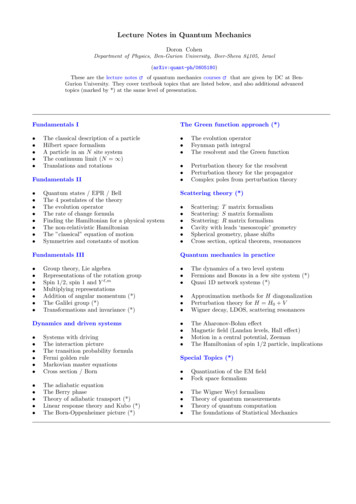
Lecture Notes in Quantum MechanicsDoron CohenDepartment of Physics, Ben-Gurion University, Beer-Sheva 84105, Israel(arXiv:quant-ph/0605180)of quantum mechanics coursesthat are given by DC at BenThese are the lecture notesGurion University. They cover textbook topics that are listed below, and also additional advancedtopics (marked by *) at the same level of presentation.Fundamentals IThe Green function approach (*) The evolution operatorFeynman path integralThe resolvent and the Green function Perturbation theory for the resolventPerturbation theory for the propagatorComplex poles from perturbation theoryThe classical description of a particleHilbert space formalismA particle in an N site systemThe continuum limit (N )Translations and rotationsFundamentals II Quantum states / EPR / BellThe 4 postulates of the theoryThe evolution operatorThe rate of change formulaFinding the Hamiltonian for a physical systemThe non-relativistic HamiltonianThe ”classical” equation of motionSymmetries and constants of motionScattering theory (*) Scattering: T matrix formalismScattering: S matrix formalismScattering: R matrix formalismCavity with leads ‘mesoscopic’ geometrySpherical geometry, phase shiftsCross section, optical theorem, resonancesFundamentals IIIQuantum mechanics in practice The dynamics of a two level systemFermions and Bosons in a few site system (*)Quasi 1D network systems (*) Approximation methods for H diagonalizationPerturbation theory for H H0 VWigner decay, LDOS, scattering resonances The Aharonov-Bohm effectMagnetic field (Landau levels, Hall effect)Motion in a central potential, ZeemanThe Hamiltonian of spin 1/2 particle, implicationsGroup theory, Lie algebraRepresentations of the rotation groupSpin 1/2, spin 1 and Y ,mMultiplying representationsAddition of angular momentum (*)The Galilei group (*)Transformations and invariance (*)Dynamics and driven systems Systems with drivingThe interaction pictureThe transition probability formulaFermi golden ruleMarkovian master equationsCross section / Born The adiabatic equationThe Berry phaseTheory of adiabatic transport (*)Linear response theory and Kubo (*)The Born-Oppenheimer picture (*)Special Topics (*) Quantization of the EM fieldFock space formalism The Wigner Weyl formalismTheory of quantum measurementsTheory of quantum computationThe foundations of Statistical Mechanics
2Opening remarksThese lecture notes are based on 3 courses in non-relativistic quantum mechanics that are given at BGU: ”Quantum 2”(undergraduates), ”Quantum 3” (graduates), and ”Selected topics in Quantum and Statistical Mechanics” (graduates).The lecture notes are self contained, and give the road map to quantum mechanics. However, they do not intend tocome instead of the standard textbooks. In particular I recommend:[1] L.E.Ballentine, Quantum Mechanics (library code: QC 174.12.B35).[2] J.J. Sakurai, Modern Quantum mechanics (library code: QC 174.12.S25).[3] Feynman Lectures Volume III.[4] A. Messiah, Quantum Mechanics. [for the graduates]The major attempt in this set of lectures was to give a self contained presentation of quantum mechanics, which is notbased on the historical ”quantization” approach. The main inspiration comes from Ref.[3] and Ref.[1]. The challengewas to find a compromise between the over-heuristic approach of Ref.[3] and the too formal approach of Ref.[1].Another challenge was to give a presentation of scattering theory that goes well beyond the common undergraduatelevel, but still not as intimidating as in Ref.[4]. A major issue was to avoid the over emphasis on spherical geometry.The language that I use is much more suitable for research with “mesoscopic” orientation.Some highlights for those who look for original or advanced pedagogical pieces: The EPR paradox, Bell’s inequality,and the notion of quantum state; The 4 postulates of quantum mechanics; Berry phase and adiabatic processes; Linearresponse theory and the Kubo formula; Wigner-Weyl formalism; Quantum measurements; Quantum computation;The foundations of Statistical mechanics. Note also the following example problems: Analysis of systems with 2or 3 or more sites; Analysis of the Landau-Zener transition; The Bose-Hubbard Hamiltonian; Quasi 1D networks;Aharonov-Bohm rings; Various problems in scattering theory.Additional topics are covered by:[5] D. Cohen, Lecture Notes in Statistical Mechanics and Mesoscopic, arXiv:1107.0568CreditsThe first drafts of these lecture notes were prepared and submitted by students on a weekly basis during 2005.Undergraduate students were requested to use HTML with ITEX formulas. Typically the text was written in Hebrew.Graduates were requested to use Latex. The drafts were corrected, integrated, and in many cases completely re-writtenby the lecturer. The English translation of the undergraduate sections has been prepared by my former student GiladRosenberg. He has also prepared most of the illustrations. The current version includes further contributions by myPhD students Maya Chuchem and Itamar Sela. I also thank my colleague Prof. Yehuda Band for some commentson the text. The arXiv versions are quite remote from the original (submitted) drafts, but still I find it appropriateto list the names of the students who have participated: Natalia Antin, Roy Azulai, Dotan Babai, Shlomi Batsri,Ynon Ben-Haim, Avi Ben Simon, Asaf Bibi, Lior Blockstein, Lior Boker, Shay Cohen, Liora Damari, Anat Daniel,Ziv Danon, Barukh Dolgin, Anat Dolman, Lior Eligal, Yoav Etzioni, Zeev Freidin, Eyal Gal, Ilya Gurwich, DavidHirshfeld, Daniel Hurowitz, Eyal Hush, Liran Israel, Avi Lamzy, Roi Levi, Danny Levy, Asaf Kidron, Ilana Kogen,Roy Liraz, Arik Maman, Rottem Manor, Nitzan Mayorkas, Vadim Milavsky, Igor Mishkin, Dudi Morbachik, ArielNaos, Yonatan Natan, Idan Oren, David Papish, Smadar Reick Goldschmidt, Alex Rozenberg, Chen Sarig, Adi Shay,Dan Shenkar, Idan Shilon, Asaf Shimoni, Raya Shindmas, Ramy Shneiderman, Elad Shtilerman, Eli S. Shutorov,Ziv Sobol, Jenny Sokolevsky, Alon Soloshenski, Tomer Tal, Oren Tal, Amir Tzvieli, Dima Vingurt, Tal Yard, UziZecharia, Dany Zemsky, Stanislav Zlatopolsky.
3ContentsFundamentals (part I)1 Introduction52 Digression: The classical description of nature93 Hilbert space134 A particle in an N site system205 The continuum limit226 Rotations28Fundamentals (part II)7 Quantum states / EPR / Bell / postulates338 The evolution of quantum mechanical states439 The non-relativistic Hamiltonian4710 Getting the equations of motion52Fundamentals (part III)11 Group representation theory6012 The group of rotations6613 Building the representations of rotations7014 Rotations of spins and of wavefunctions7315 Multiplying representations8116 Galilei group and the non-relativistic Hamiltonian9017 Transformations and invariance92Dynamics and Driven Systems18 Transition probabilities9819 Transition rates10220 The cross section in the Born approximation10421 Dynamics in the adiabatic picture10722 The Berry phase and adiabatic transport11123 Linear response theory and the Kubo formula11724 The Born-Oppenheimer picture120The Green function approach25 The propagator and Feynman path integral12126 The resolvent and the Green function12527 Perturbation theory13528 Complex poles from perturbation theory140
4Scattering Theory29 The plane wave basis14330 Scattering in the T -matrix formalism14631 Scattering in the S-matrix formalism15332 Scattering in quasi 1D geometry16333 Scattering in a spherical geometry171QM in Practice (part I)34 Overview of prototype model systems18035 Discrete site systems18136 Two level dynamics18237 A few site system with Bosons18638 A few site system with Fermions18939 Boxes and Networks191QM in Practice (part II)40 Approximation methods for finding eigenstates19641 Perturbation theory for the eigenstates20042 Beyond perturbation theory20643 Decay into a continuum21044 Scattering resonances219QM in Practice (part III)45 The Aharonov-Bohm effect22346 Motion in uniform magnetic field (Landau, Hall)23147 Motion in a central potential24048 The Hamiltonian of a spin 1/2 particle24449 Implications of having ”spin”247Special Topics50 Quantization of the EM Field25151 Quantization of a many body system25652 Wigner function and Wigner-Weyl formalism26753 Quantum states, operations and measurements27554 Theory of quantum computation28755 The foundation of statistical mechanics297
5Fundamentals (part I)[1] Introduction [1.1] The building blocks of the universeThe universe consists of a variety of particles which are described by the ”standard model”. The known particles aredivided into two groups: Quarks: constituents of the proton and the neutron, which form the 100 nuclei known to us.Leptons: include the electrons, muons, taus, and the neutrinos.The interaction between the particles is via fields (direct interaction between particles is contrary to the principlesof the special theory of relativity). These interactions are responsible for the way material is ”organized”. Weshall consider in this course the electromagnetic interaction. The electromagnetic field is described by the Maxwellequations. Within the framework of the ”standard model” there are additional gauge fields that can be treated onequal footing. In contrast the gravity field has yet to be incorporated into quantum theory. [1.2] A particle in an electromagnetic fieldThis section is inteted for 3rd year BSc Physics students: its purpose is to place this course in the context of classicalanalytical mechanics. Those who do not have this eduction can skip sections [1.2]-[1.3]-[1.4]. A terse summary ofclassical mechanics is provided in lecture [2], and can be skipped as well.Within the framework of classical electromagnetism, the electromagnetic field is described by the scalar potential V (x) and the vector potential A(x).In addition one defines: B A 1 A VE c t(1.1)We will not be working with natural units in this course, but from now on we are going to absorb the constants c ande in the definition of the scalar and vector potentials:eA A,ceB B,ceV V(1.2)eE EIn classical mechanics, the effect of the electromagnetic field is described by Newton’s second law with the Lorentzforce. Using the above units convention we write:ẍ 1(E B v)m(1.3)The Lorentz force dependents on the velocity of the particle. This seems arbitrary and counter intuitive, but we shallsee in the future how it can be derived from general and fairly simple considerations.In analytical mechanics it is customary to derive the above equation from a Lagrangian. Alternatively, one can use aLegendre transform and derive the equations of motion from a Hamiltonian: H p Hṗ xẋ (1.4)
6where the Hamiltonian is:H(x, p) 1(p A(x))2 V (x)2m(1.5)The Hamiltonian that describes a system of several charged particles in 3 dimensional space, including the electromagnetic field in the Coulomb gauge, can be written as follows:ZX 1X ei ej122H(r, p, A, E) (E c2 ( A)2 )d3 x(pi ei A(ri )) 2m r r 8πiiji(1.6)hijiThe canonical coordinates of the particles are (ri , pi ), and the canonical coordinates of the radiations field are (A, E ).The magnetic field is defined as B A. One can define an electrostatic electric field Ek , and express the secondterm as an integral over Ek2 /(8π).The units of E as well as the prefactor 1/(8π) are determined via Coulomb law as in the Gaussian CGI convention.The units of A are determined as in the SI convention, namely, we do not make here the replacement A 7 (1/c)A,and therefore the equations of motion for the radiation field imply that E Ȧ. Accordingly B and E do not havethe same units, and the Lorentz force formula does not included (1/c) prefactor.In the absence of particles the radiation term of the Hamiltonian describes waves that have a dispersion relationω c k . The strength of the interaction is determined by the coupling constants ei . Assuming that all the particleshave elementary charge ei e, it follows that after canonical quantization (see below) the above Hamiltonian ischaracterized by a single dimensionless coupling constant e2 /( c), which is knows as the “fine-structure constant”. [1.3] Canonical quantizationThe historical method of deriving the quantum description of a system is canonical quantization. In this method weassume that the particle is described by a ”wave function” that obeys the equation: i Ψ(x) H x, i Ψ(x) t x(1.7)This seems arbitrary and counter-intuitive. In this course we shall abandon the historical approach. Instead we shallconstruct quantum mechanics using simple heuristic considerations. Later we shall see that classical mechanics canbe obtained as a special limit of the quantum theory. [1.4] Second quantizationThe method for quantizing the electromagnetic radiation field is to write its Hamiltonian as a sum of harmonicoscillators (normal modes) and then to quantize the oscillators. It is exactly the same as finding the normal modesof spheres connected with springs. Every normal mode has a characteristic frequency. The ground state of the field(all the oscillators are in the ground state) is called the ”vacuum state”. If a specific oscillator is excited to level n,we say that there are n photons with frequency ω in the system.A similar formalism is used to describe a many particle system. A vacuum state and occupation states are defined.This formalism is called ”second quantization”. A better name would be ”formalism of quantum field theory”. Oneimportant ingredient of this formulation is the distinction between fermions and bosons.In the first part of this course we regard the electromagnetic field as a classical entity, where V (x), A(x) are given asan input. The distinction between fermions and bosons will be obtained using the somewhat unnatural language of”first quantization”.
7 [1.5] Definition of massThe ”gravitational mass” is defined using a weighting apparatus. Since gravitational theory is not includes in thiscourse, we shall not use that definition. Another possibility is to define ”inertial mass”. This type of mass is determinedby considering the collision of two bodies:m1 v1 m2 v2 m1 u1 m2 u2(1.8)Accordingly one can extract the mass ratio of the two bodies:m1u2 v 2 m2u1 v 1(1.9)In order to give information on the inertial mass of an object, we have to agree on some reference mass, say the”kg”, to set the units. (less arbitrary would be to take the mass of the proton as the reference). Anyway, within theframework of quantum mechanics the above Newtonian definition of inertial mass will not be used. Rather we definemass in an absolute way, that does not require to fix a reference mass. We shall define mass as a parameter in the”dispersion relation”.The dispersion relation.– It is possible to prepare a ”monochromatic” beam of particles (say electrons) that allhave the same velocity, and the same De-Broglie wavelength. The velocity of the particles can be measured by usinga pair of rotating circular plates (discs). The wavelength of the beam can be measured using a diffraction grating.We define the momentum of the moving particles (”wave number”) as:p 2π/wavelength(1.10)It is possible to find (say by an experiment) the relation between the velocity of the particle and its momentum. Thisrelation is called the ”dispersion relation”. Here is a plot of what we expect to observe:cvpmpFor low (non relativistic) velocities the relation is approximately linear:v cppc 2(mc )2 (cp)21pm(1.11)This relation defines the ”mass” parameter. The implied units of mass are[m] TL2(1.12)If we use arbitrary units for measuring mass, say ”kg”, then the conversion prescription is: secondm[kg] m,meter2 where is known as the Planck constant.h2π(1.13)
8 [1.6] Semiclassical perspectiveWithin the semi-classical picture we specify the state of a particle using two dynamical variables (x, p). It is aphenomenological observation that the momentum (as defined in the previous section) can be increased by applying“force”. In fact we can define the term force in a semi-Newtonian way:dp Fdt V (x) x(1.14)where V (x) is a function that describes the field of force. Similarly we can define kinetic-energy-function K(p) fromwhich the dispersion relation is derived:dx v(p) dt K(p) p(1.15)The standard dispersion relation isK(p) pp2(mc2 )2 (cp)2 mc2 2m(1.16)The latter expression is the non-relativistic approximation. We can define Hamiltonian formally as followsH(x, p) K(p) V (x)(1.17)and derive from it the equations of motion. We define the energy asE H(x, p)(1.18)It is easily verified that E is a constant of motion (dE/dt 0). The energy has units of frequency. The conversion toSI units is: Ekg · meter2second2 E1second (1.19) [1.7] SpinApart from the degrees of freedom of being in space, the particles also have an inner degree of freedom called ”spin”.We say that a particle has spin s if its inner degree of freedom is described by a representation of the rotations groupof dimension 2s 1. For example, ”spin 12 ” can be described by a representation of dimension 2, and ”spin 1” can bedescribed by a representation of dimension 3. In order to make this abstract statement clearer we will look at severalexamples. Electrons have spin 21 , hence 180o difference in polarization (”up” and ”down”) means orthogonality. Photons have spin 1, hence 90o difference in linear polarizations means orthogonality.If we position two polarizers one after the other in the angles that were noted above, no particles will pass through.We see that an abstract mathematical consideration (representations of the rotational group) has very realistic consequences.
9[2] Digression: The classical description of nature [2.1] The electromagnetic fieldThe electric field E and the magnetic field B can be derived from the vector potential A and the electric potential V :E V 1 Ac t(2.1) B AThe electric potential and the vector potential are not uniquely determined, since the electric and the magnetic fieldsare not affected by the following changes:1 Λc tA 7Ã A ΛV 7 Ṽ V (2.2)where Λ(x, t) is an arbitrary scalar function. Such a transformation of the potentials is called ”gauge”. A special caseof ”gauge” is changing the potential V by an addition of a constant.Gauge transformations do not affect the classical motion of the particle since the equations of motion contain onlythe derived fields E, B.i1 hed2 x eE B ẋdt2mc(2.3)This equation of motion can be derived from the Lagrangian:L(x, ẋ) 1 2 emẋ ẋA(x, t) eV (x, t)2c(2.4)Or, alternatively, from the Hamiltonian:H(x, p) 1e(p A)2 eV2mc(2.5) [2.2] The Lorentz TransformationThe Lorentz transformation takes us from one reference frame to the other. A Lorentz boost can be written in matrixform as: γ γβ 0 0 γβ γ 0 0 S 00 1 0 00 0 1 (2.6)where β is the velocity of our reference frame relative to the reference frame of the lab, andγ p11 β2(2.7)
10We use units such that the speed of light is c 1. The position of the particle in space is: t x x yz(2.8)and we write the transformations as:x0 Sx(2.9)We shall see that it is convenient to write the electromagnetic field as: 0 E1E2E30B3 B2 EF 1E2 B3 0B1 E3 B2 B1 0 (2.10)We shall argue that this transforms as:F 0 SF S 1(2.11)or in terms of components:E10 E1B10 B1E20 γ(E2 βB3 ) B20 γ(B2 βE3 )E30 γ(E3 βB2 ) B30 γ(B3 βE2 ) [2.3] Momentum and energy of a particleLet us write the displacement of the particle as: dt dx dx dydz (2.12)We also define the proper time (as measured in the particle frame) as:dτ 2 dt2 dx2 dy 2 dz 2 (1 vx 2 vy 2 vz 2 )dt2(2.13)or:dτ p1 v 2 dt(2.14)The relativistic velocity vector is:u dx,dτ[u2t u2x u2y u2z 1](2.15)
11It is customary to define the non-canonical momentum as p p mu x pypz (2.16)According to the above equations we have: 2 p2x p2y p2z m2(2.17)and write the dispersion relation:pm 2 p2pv pm2 p2 (2.18)We note that for non-relativistic velocities pi mvi for i 1, 2, 3 while: mdtdτ m1 v21 m mv 2 . . .2(2.19) [2.4] Equations of motion for a particleThe non-relativistic equations of motion for a particle in an electromagnetic field are:md vdt eE eB v(2.20)The right hand side is the so-called Lorentz force f . It gives the rate of change of the non-canonical momentum. Therate of change of the associated non-canonical energy E isd dt f · v eE · v(2.21)The electromagnetic field has equations of motion of its own: the Maxwell equations. We shall see shortly thatMaxwell equations are Lorentz invariant. But what Newton’s second law as written above is not Lorentz invariant.In order for the Newtonian equations of motion to be Lorentz invariant we have to adjust them. It is not difficult tosee that the obvious required revision is:mdudτ eF u(2.22)To prove the invariance under the Lorentz transformation we write:ddeee 0 0du0 (Su) S u S F u SF S 1 (Su) F udτdτdτmmmHence we have deduced the transformation F 0 SF S 1 of the electromagnetic field.(2.23)
12 [2.5] Equations of motion of the fieldBack to the Maxwell equations. A simple way of writing them is † F 4πJ †(2.24)where the derivative operator , and the four-current J, are defined as: t x y z † ,,, t x y z (2.25)and: ρ J J x JyJz J† (ρ, Jx , Jy , Jz )(2.26)The Maxwell equations are invariant because J and transform as vectors. For more details see Jackson. Animportant note about notations: in this section we have used what is called a ”contravariant” representation for thecolumn vectors. For example u column(ut , ux , uy , uz ). For the ”adjoint” we use the ”covariant” representationu row(ut , ux , uy , uz ). Note that u† u (ut )2 (ux )2 (uy )2 (uz )2 is a Lorentz scalar.
13[3] Hilbert space [3.1] Linear algebraIn Euclidean geometry, three dimensional vectors can be written as: u u1 e1 u2 e2 u3 e3(3.1)Using Dirac notation we can write the same as: ui u1 e1 i u2 e2 i u3 e3 i(3.2)We say that the vector has the representation: u1 ui 7ui u2 u3(3.3)The operation of a linear operator A is written as vi A ui which is represented by: v1A11 A12 A13u1 v2 A21 A22 A23 u2 v3A31 A32 A33u3(3.4)or shortly as vi Aij uj . Thus a linear operator is represented by a matrix:A 7 Aij A11 A12 A13 A21 A22 A23 A31 A32 A33(3.5) [3.2] Orthonormal basisWe assume that an inner product hu vi has been defined. From now on we assume that the basis has been chosen tobe orthonormal:hei ej i δij(3.6)In such a basis the inner product (by linearity) can be calculated as follows:hu vi u 1 v1 u 2 v2 u 3 v3(3.7)It can also be easily proved that the elements of the representation vector can be calculated as follows:uj hej ui(3.8)And for the matrix elements we can prove:Aij hei A ej i(3.9)
14 [3.3] Completeness of the basisIn Dirac notation the expansion of a vector is written as: ui e1 ihe1 ui e2 ihe2 ui e3 ihe3 ui(3.10)which implies1 e1 ihe1 e2 ihe2 e3 ihe3 (3.11)Above 1 7 δij stands for the identity operator, and P j ej ihej are called ”projector operators”, 1 0 01 7 0 1 0 ,0 0 1 1 0 0P 1 7 0 0 0 ,0 0 0 0 0 0P 2 7 0 1 0 ,0 0 0 0 0 0P 3 7 0 0 0 ,0 0 1(3.12)Now we can define the ”completeness of the basis” as the requirementXPjX j ej ihej 1(3.13)jFrom the completeness of the basis it follows e.g. that for any operatorA "X#Pi XXXA P j ei ihei A ej ihej ei iAij hej iji,j(3.14)i,j [3.4] OperatorsIn what follows we are interested in ”normal” operators that are diagonal in some orthonormal basis. Say that wehave an operator A. By definition, if it is normal, there exists an orthonormal basis { ai} such that A is diagonal.Hence we writeA X aiaha aXaP a(3.15)aIn matrix representation it means: 1 0 00 0 00 0 0a1 0 0 0 a2 0 a1 0 0 0 a2 0 1 0 a3 0 0 0 0 0 00 0 00 0 10 0 a3(3.16)PIt is useful to define what is meant by B̂ f (Â) where f () is an arbitrary function. Assuming that  aiaha , itPfollows by definition that B̂ aif (a)ha . Another useful rule to remember is that if A ki B ki for some completebasis k, then it follows by linearity that A ψi B ψi for any vector, and therefore A B.With any operator A, we can associate an “adjoint operator” A† . By definition it is an operator that satisfies thefollowing relation:hu Avi hA† u vi(3.17)
15If we substitute the basis vectors in the above relation we get the equivalent matrix-style definition(A† )ij A ji(3.18)If A is normal then it is diagonal in some orthonormal basis, and then also A† is diagonal in the same basis. It followsthat a normal operator has to satisfy the necessary condition A† A AA† . As we show below this is also a sufficientcondition for ”normality”.We first consider Hermitian operators, and show that they are ”normal”. By definition they satisfy A† A. If wewrite this relation in the eigenstate basis we deduce after one line of algebra that (a b)ha bi 0, where a and b areany two eigenvalues. If follows (considering a b) that the eigenvalues are real, and furthermore (considering a 6 b)that eigenvectors that are associate with different eigenvalues are orthogonal. This is called the spectral theorem: onecan find an orthonormal basis in which A is diagonal.We now consider a general operator Q. Always we can write it asQ A iB,with A 1(Q Q† ),2and B 1(Q Q† )2i(3.19)One observes that A and B are Hermitian operators. It is easily verified that Q† Q QQ† iff AB BA. It followsthat there is an orthonormal basis in which both A and B are diagonal, and therefore Q is a normal operator.We see that an operator is normal iff it satisfies the commutation Q† Q QQ† and iff it can be written as a functionf (H) of an Hermitian operator H. We can regard any H with non-degenerate spectrum as providing a specificationof a basis, and hence any other operator that is diagonal in that basis can be expressed as a function of this H.Of particular interest are unitary operators. By definition they satisfy U † U 1, and hence they are ”normal” andcan be diagonalized in an orthonormal basis. Hence their eigenvalues satisfy λ r λr 1, which means that they can bewritten as:U X rieiϕr hr eiH(3.20)rwhere H is Hermitian. This is an example for the general statement that any normal operator can be written as afunction of some Hermitian operator H. [3.5] Conventions regarding notationsIn Mathematica there is a clear distinction between dummy indexes and fixed values. For example f (x ) 8 meansthat f (x) 8 for any x, hence x is a dummy index. But if x 4 then f (x) 8 means that only one element of thevector f (x) is specified. Unfortunately in the printed mathematical literature there are no clear conventions. Howeverthe tradition is to use notations such as f (x) and f (x0 ) where x and x0 are dummy indexes, while f (x0 ) and f (x1 )where x0 and x1 are fixed values. Thus 2 35 7 5for i0 2 and j0 1Aij Ai0 j0(3.21)Another typical example isTx,k hx ki matrixΨ(x) hx k0 i column(3.22)(3.23)In the first equality we regard hx ki as a matrix: it is the transformation matrix form the position to the momentumbasis. In the second equality we regard the same object (with fixed k0 ) as a column, or as a ”wave-function”.
16We shall keep the following extra convention: The ”bra” indexes would appear as subscripts (used for representation),while the ”ket” indexes would appear as superscripts (reserved for the specification of the state). For example:Y m (θ, ϕ) hθ, ϕ mi spherical harmonicsϕn (x) hx ni harmonic oscillator eigenfunctionsψn hn ψi representation of wavefunction in the n basis(3.24)(3.25)(3.26)Sometime it is convenient to use the Einstein summation convention, where summation over repeated dummy indexesis implicit. For example:Xhθ, ϕ mih m f i f m Y m (θ, ϕ)f (θ, ϕ) (3.27) mIn any case of ambiguity it is best to translate everything into Dirac notations. [3.6] Change of basisDefinition of T :Assume we have an ”old” basis and a ”new” basis for a given vector space. In Dirac notation:old basisnew basis { i 1i, i 2i, i 3i, . . . }{ n 1i, n 2i, n 3i, . . . }(3.28)The matrix Ti,n whose columns represent the vectors of the new basis in the old basis is called the ”transformationmatrix from the old basis to the new basis”. In Dirac notation this may be written as: ni XTi,α ii(3.29)iIn general, the bases do not have to be orthonormal. However, if they are orthonormal then T must be unitary andwe haveTi,n hi ni(3.30)In this section we will discuss the general case, not assuming orthonormal basis, but in the future we will always workwith orthonormal bases.Definition of S:If we have a vector-state then we can represent it in the old basis or in the new basis: ψi Xψi ii(3.31)i ψi Xψ̃n ninSo, the change of representation can be written as:ψ̃n XiSn,i ψi(3.32)
17Or, written abstractly:ψ̃ Sψ(3.33)The transformation matrix S T 1 reflects that change of basis can be regarded as an active operation on the stateof the system. For example, if T represents forward translation of the axes (change of basis, passive point of view),then S represents a backward translation of the system (operation, active point of view).Similarity Transformation:A unitary operation can be represented in either the new basis or the old basis:ϕi XAi,j ψj(3.34)iϕ̃n XÃn,m ψ̃mnThe implied transformation between the representations is:Ã SAS 1 T 1 AT(3.35)This is called a similarity transformation. [3.7] Non-orthonormal basis and the dual basisGiven an arbitrary basis that is not necessarily orthonormal, we define a metric gij hi ji such
Lecture Notes in Quantum Mechanics Doron Cohen Department of Physics, Ben-Gurion University, Beer-Sheva 84105, Israel (arXiv:quant-ph/0605180) These are thelecture notes of quantum mechanicscourses that are given by DC at Ben-Gurion University. They cover textbook t