Transcription
Financial ForecastingCHAPTER 5After studying this chapter, you should be able to:1.Explain how the “percent of sales” method is used to develop pro forma financialstatements and how to construct such statements in Excel.2.Use circular references to perform iterative calculations.3.Use the TREND function for forecasting sales or any other trending variables.4.Perform a regression analysis with Excel’s built-in regression tools.5.Determine if a variable is statistically significant in a regression analysis.Forecasting is an important activity for a wide variety of business people. Nearly all of thedecisions made by financial managers are made on the basis of forecasts of one kind oranother. For example, in Chapter 3 we’ve seen how the cash budget can be used to forecastshort-term borrowing and investing needs. Every item in the cash budget is itself a forecast.In this chapter, we will examine several methods of forecasting. The first, the percent ofsales method, is the simplest. We will also look at more advanced techniques, such asregression analysis.141
CHAPTER 5: Financial ForecastingThe Percent of Sales MethodForecasting financial statements is important for a number of reasons. Among these areplanning for the future and providing information to the company’s investors. The simplestmethod of forecasting income statements and balance sheets is the percent of sales method.This method has the added advantage of requiring relatively little data to make a forecast.The fundamental premise of the percent of sales method is that some, but not all, incomestatement and balance sheet items maintain a constant relationship with the level of sales.For example, if the cost of goods sold has averaged 65% of sales over the last several years,we would assume that this relationship would hold for the next year. If sales are expectedto be 10 million next year, our cost of goods forecast would be 6.5 million(10 million 0.65 6.5 million).Of course, this method assumes that the forecasted level of sales is already known. There aretwo primary methods of forecasting sales. The top-down method relies on forecasts ofmacroeconomic variables (e.g., GDP, inflation rates, etc.) and of the condition of theindustry as a whole. These expectations are then converted into a sales forecast for the entirefirm, and sales targets for each division or product. The bottom-up method involvesdiscussions with customers to determine the expected demand for each product andexpectations regarding prices, which are then summed to calculate a firm-wide salesforecast. Of course, firms can use a combination of the two methods. We will take the salesforecast as a given.Forecasting the Income StatementAs an example of income statement forecasting, consider the Elvis Products International(EPI) statements that you created in Chapter 2. The income statement is recreated here inExhibit 5-1. Recall that we have used a custom number format to display this data inthousands of dollars, but that the full-precision numbers are there. Open the workbook thatyou created for Chapter 2, and make a copy of the Income Statement worksheet. Rename thenew worksheet to Pro Forma Income Statement.1The level of detail that you have in an income statement will affect the number of itemsthat will fluctuate directly with sales. In general, we will proceed through the incomestatement line by line asking the question, “Is it likely that this item will changeproportionally with sales?” If the answer is yes, then we calculate the percentage of salesand multiply the result by the sales forecast for the next period. Otherwise, we will takeone of two actions: Leave the item unchanged, or use other information to change1. Pro forma is a Latin word that, for our purposes, can be interpreted to mean “as if.” That is, theseforecasted financial statements are presented as if the forecast time period has already happened.142
The Percent of Sales Methodthe item.2 If you don’t know the answer, then you can create a chart that compares the itemto sales over the last several quarters or years. It should be obvious if there is arelationship, though you may need to use some of the statistical tools, discussed onpage 154, to determine the form of the relationship.EXHIBIT 5-1EPI’S INCOME STATEMENTS FOR 2010 AND 2011For EPI, only one income statement item will clearly change with sales: the cost of goodssold. Another item, SG&A (selling, general, and administrative) expense, is an aggregationof many things, some of which will probably change with sales and some that won’t. For ourpurposes we choose to believe that, on balance, SG&A will change along with sales.Changes in the other items are not directly related to a change in sales in the short term.Depreciation expense, for example, depends on the amount and age of the firm’s fixedassets. Interest expense is a function of the amount and maturity structure of debt in thefirm’s capital structure. These items may, and probably will, change but we will needadditional information. Taxes depend directly on the firm’s taxable income, though thisindirectly depends on the level of sales. All of the other items on the income statement arecalculated directly.2. For example, if you know that the lease for the company’s headquarters building has a scheduledincrease, then you should be sure to include this information in your forecast for fixed costs.143
CHAPTER 5: Financial ForecastingBefore getting started with the forecast, insert a column to the left of column B. Select a cellin column B and click the Insert button on the Home tab and then choose Insert SheetColumns. Note that a Smart Tag will appear that will give you three choices: (1) FormatSame As Left; (2) Format Same As Right; or (3) Clear Formatting. Choose the secondoption so that the custom number formats and column width will automatically be applied.So that we can experiment later if we choose, enter 40% for the tax rate in B18.To generate our income statement forecast, we first determine the percentage of sales foreach of the prior years for each item that changes. In this case, for 2011 we have:Cost of Goods Sold 2011Percentage of Sales 3,250,000--------------------------- 0.8442 84.42%3,850,000SG&A Expense 2011Percentage of Sales 330,300------------------------ 0.0858 8.58%3,850,000The 2010 percentages (83.45% and 6.99%, respectively) can be found in exactly the samemanner. We now calculate the average of these percentages and use this average as ourestimate of the 2012 percentage of sales. The forecast is then found by multiplying thesepercentages by next year’s sales forecast. Assuming that sales are forecasted to be 4,300,000 in 2012 we have:Cost of Goods Sold2012 Forecast 4,300,000 0.8393 3,609,108SG&A Expense 2012Forecast 4,300,000 0.0779 334,803Exhibit 5-2 shows a forecast of the complete 2012 income statement. To create this forecastin your worksheet, in B4 enter: 2012.3 Because the 2012 income statement will becalculated in exactly the same way as 2011, the easiest way to proceed is to copy C5:C15into B5:B15. This will save you from having to enter formulas to calculate subtotals (e.g.,EBIT) and will apply the cell borders. Insert a row above row 17, and in A16 type:*Forecast.First, in B5 enter the sales forecast: 4,300,000. Now, we can calculate the 2012 cost ofgoods forecast in B6 with the formula: AVERAGE(C6/C 5,D6/D 5)*B 5. Thisformula calculates the average of the cost of goods as a percentage of sales for the last two3. We have chosen to apply a custom format so that the number has an asterisk to indicate a footnotethat informs the reader that these are forecasts. The custom format is #”*”.144
The Percent of Sales Methodyears and then multiplies it by the sales forecast. The result should be as shown above. Nowcopy this formula to B8 to get the forecast for SG&A expense.EXHIBIT 5-2PERCENT OF SALES FORECAST FOR 2012Instead of performing the entire calculation in cells B6 and B8, we could have used a helpercolumn. A helper column is used to do intermediate calculations and is sometimes useful. Inthis case, we could have calculated the average percentage of sales for each item in, say,column K. We would then use these values to perform the final calculation in column B. Forexample, K6 might contain the formula: AVERAGE(C6/C 5,D6/D 5). Then theformula in B6 would be: K6*B 5. This technique would allow you to easily see theaverage percentages (as in a common-size income statement) that are being used to generatethe forecast. Although this might be useful, it can be an inefficient use of the spreadsheetunless it is necessary.Assume that we do not have any information regarding changes in fixed expenses, so copythe value from C9. However, we have been informed that the firm intends to invest 50,000in fixed assets in 2012. This will cause depreciation expense to rise by 5,000. We need todocument this assumption, so in A20 type: Additional Depreciation, and in B20enter: 5,000. We will come back to add a formula in B20 in the next section. Don’t forgetto apply the same custom number format to this cell that we used in the others.145
CHAPTER 5: Financial ForecastingThe formula to calculate depreciation expense in B10 is: C10 B20. Because we don’t yetknow how the firm will finance these investments, leave the interest expense at the samelevel as 2011. To calculate the taxes, in B14, use the formula: B19*B13. Your worksheetshould now look like the one in Exhibit 5-2.Forecasting Assets on the Balance SheetWe can forecast the balance sheet in exactly the same way as the income statement, withsome major exceptions. For those items that can be expected to vary directly with sales, ourformulas will be similar to those we have already seen. We will explain how to handle theother items below.Create the percent of sales balance sheet for 2012 by selecting column B and inserting a newcolumn. In B4 type the label: 2012. As before, apply a custom number format to display anasterisk after the number. Like we did with the income statement, we will move, line by line,through the balance sheet to determine which items will vary with sales.The firm’s cash balance is the first, and perhaps the most difficult, item with which we needto work. Does the cash balance vary, in constant proportion, with sales? Your first responsemight be, “Of course it does. As the firm sells more goods, it accumulates cash.” This line ofreasoning neglects two important facts. The firm has other things to do with its cash besidesaccumulating it, and because cash is a low-return asset, firms should seek to minimize theamount of their cash balance.4 For these reasons, even though the cash balance will probablychange, it probably will not change by the same percentage as sales. Therefore, we willsimply use the cash balance from 2011 as our forecast, so enter: C5 into cell B5.The next two items, accounts receivable and inventory, are much easier. Both of these arelikely to fluctuate roughly in proportion to sales. Using the same methodology that we usedfor the pro forma income statement, we will find the average percentage of sales for the pasttwo years and multiply that amount by our sales forecast for 2012. For accounts receivable,the formula in B6 is: AVERAGE(C6/'Income Statement'!B 5,D6/'IncomeStatement'!C 5)*'Pro Forma Income Statement'! B 5. Instead of typingthe references to the income statement, it is easier to insert them by displaying both theincome statement and balance sheet and selecting the appropriate cells with the mouse. Clickthe View tab and select New Window. This will create an additional view of the workbook.Next, click on the Arrange All button and choose how you would like the worksheetsarranged. In the second view, change to the Income Statement worksheet. Now that bothworksheets are visible, it is easier to select cells. Because we will use the same formula for4. Within reason, of course. Firms need some amount of cash to operate, but the amount needed doesnot necessarily vary directly with the level of sales.146
The Percent of Sales Methodinventory, we can simply copy this formula down to B7. Total current assets in B8 is acalculated value, so we can copy the formula directly from cell C8.In B9, we have the 2012 gross plant and equipment. This is the historical purchase price ofthe buildings and equipment that the firm owns. As noted earlier, the firm plans to make netnew investments of 50,000 in 2012. We will document this assumption by entering NetAddition to Plant and Equipment in A28 and 50,000 in B28. The formula in B9is: C9 B28. Note that this increase is not necessarily due to the expected increase in sales.Although gross fixed assets may rise or fall in any given year, most companies alwaysoperate with spare capacity so the changes are not, in the short run, directly related to sales.We now need to calculate the additional depreciation. We will assume that the expected lifeof the new equipment is 10 years and that it will be depreciated using the straight linemethod to a salvage value of zero. In A29 enter the label: Life of New Equipment inYears, and in B29 enter 10. In A30 enter: New Depreciation (Straight Line),and in B30 enter the formula: B28/B29. The additional depreciation expense will be 5,000. Now, return to the pro forma income statement where we will enter a formula inB20: 'Pro Forma Balance Sheet'!B30. This last step allows us to change theamount of the new investment and have the additional depreciation expense reflected on thepro forma income statement.Now, return to the pro forma balance sheet. Accumulated depreciation will definitelyincrease in 2012 but not because of the forecasted change in sales. Instead, accumulateddepreciation will increase by the amount of the depreciation expense for 2012. To determinethe accumulated depreciation for 2012, we will add 2012’s depreciation expense to 2011’saccumulated depreciation. The formula is: C10 'Pro Forma Income Statement'!B10.To complete the asset side of the balance sheet, we note that both net fixed assets and totalassets are calculated values. We can simply copy the formulas from C11:C12 and paste theminto B11:B12.Forecasting Liabilities on the Balance SheetOnce the assets are completed, the rest of the balance sheet is comparatively simple becausewe can mostly copy formulas already entered. Before continuing, however, we need todistinguish among the types of financing sources. We have already seen that the types offinancing that a firm uses can be divided into three categories: Current liabilities Long-term liabilities Owner’s equityThese categories are not sufficiently distinguished for our purposes here. Instead, we willdivide the liabilities and equity of a firm into two categories:147
CHAPTER 5: Financial Forecasting Spontaneous sources of financing—These are the sources of financing thatarise during the ordinary course of doing business. One example isaccounts payable. After a credit account is established with a supplier, noadditional work is required to obtain credit; it just happens spontaneouslywhen the firm makes a purchase. Note that not all current liabilities arespontaneous sources of financing (e.g., short-term notes payable, longterm debt due in one year). Discretionary sources of financing—These are the financing sources thatrequire a large effort on the part of the firm to obtain. In other words, thefirm must make a conscious decision to obtain these funds. Furthermore,the firm’s upper-level management will use its discretion to determine theappropriate type of financing to use. Examples of this type of financinginclude any type of bank loan, bonds, preferred stock, and common stock(but not retained earnings).Generally speaking, spontaneous sources of financing can be expected to vary directly withsales. Changes in discretionary sources, on the other hand, will not have a direct relationshipwith changes in sales. We always leave discretionary sources of financing unchanged forreasons that will soon become clear.Returning now to our forecasting problem, the first item to consider is accounts payable. Asnoted above, accounts payable is a spontaneous source of financing and will, therefore,change directly with sales. To enter the formula, all that is necessary is to copy the formulafrom one of the other items that we have already completed. Copy the contents of B6 (or B7,it doesn’t matter which) and paste it into B14. The result should indicate a forecastedaccounts payable of 189.05.The next item to consider is the short-term notes payable. Because this is a discretionarysource of financing, we will leave it unchanged from 2011. In reality, we might handle thisitem differently if we had more information. For example, if we knew that the notes wouldbe retired before the end of 2012, we would change our forecast to zero. Alternatively, if thepayments on the notes include both principal and interest, our forecast would be the 2011amount less principal payments that we expect to make in 2012. Because we are leaving itunchanged, the formula in B15 is: C15.If we assume that the “other current liabilities” item represents primarily accrued expenses,then it is a spontaneous source of financing. We can, therefore, simply copy the formulafrom B14 and paste it into B16. The forecasted amount is 163.38.Long-term debt, in B18, and common stock, in B20, are both discretionary sources offinancing. We will leave these balances unchanged from 2011. In B18 the formula is: C18and in B20 the formula is: C20.148
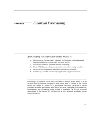
The Percent of Sales MethodThe final item that we must consider is retained earnings. Recall that retained earningsaccumulates over time. That is, the balance in any year is the accumulated amount that hasbeen added in previous years plus any new additions. The amount that will be added toretained earnings is given by:Change in Retained Earnings Net Income – Dividendswhere the dividends are those paid to both the common and preferred stockholders. Theformula for retained earnings will require that we reference forecasted 2012 net income fromthe income statement and the dividends from the statement of cash flows (see Exhibit 2-7, page59). Note that we are assuming that 2012 dividends will be the same as the 2011 dividends.We can reference these cells in exactly the same way as before, so the formula is: C21 'pro forma Income Statement'!B15 'Statement of Cash Flows'!B19.The results should show that we are forecasting retained earnings to be 297.04 in 2012.At this point, you should go back and calculate the subtotals in B17, B19, and B22. Finally,we calculate the total liabilities and owner’s equity in B23 with B19 B22.Discretionary Financing NeededSharp-eyed readers will notice that our pro forma balance sheet does not balance. Althoughthis appears to be a serious problem, it actually represents one of the purposes of the proforma balance sheet. The difference between total assets and total liabilities and owner’sequity is referred to as discretionary financing needed (DFN, also called additional fundsneeded or required new funds). In other words, this is the amount of discretionary financingthat the firm thinks it will need to raise in the next year. Because of the amount of time andeffort required to raise these funds, it is important that the firm be aware of its needs well inadvance. The pro forma balance sheet fills this need. Frequently, the firm will find that it isforecasting a higher level of assets than liabilities and equity. In this case, the managerswould need to arrange for more liabilities and/or equity to finance the level of assets neededto support the volume of sales expected. This is referred to as a deficit of discretionary funds.If the forecast shows that there will be a higher level of liabilities and equity than assets, thefirm is said to have a surplus of discretionary funds. Remember that, in the end, the balancesheet must balance. The “plug figure” necessary to make this happen is the DFN.We should add an extra line at the bottom of the pro forma balance sheet to calculate theDFN. Type Discretionary Financing Needed in A25, and in B25 add theformula B12-B23. This calculation tells us that EPI expects to need 38,119.50(displayed as 38.12 with the custom number format) more in discretionary funds tosupport its forecasted level of assets. In this case, EPI is forecasting a deficit ofdiscretionary funds. Apply the custom number format to this number and to the rest of thebalance sheet.149
CHAPTER 5: Financial ForecastingEXHIBIT 5-3EPI’S PRO FORMA BALANCE SHEET FOR 2012To make clear that this amount is a deficit (note that the sign is the opposite of what mightbe expected when using that word), we can have Excel inform us whether we will havea surplus or deficit of discretionary funds. Use an IF statement and realize that if the DFNis a positive number, then we have a deficit; otherwise we have a surplus or DFN iszero. So the formula in C25 is: IF(B25 0,"Deficit", IF(B25 0,"Surplus","Balanced")).5 Your balance sheet should now resemble that in Exhibit 5-3.5. You could also design a custom number format. One possible format is: #,###.00,"Deficit";#,###.00," Surplus". The benefits of this approach are that you don’t need touse a separate cell and you don’t need to enter a formula.150
Using Iteration to Eliminate DFNUsing Iteration to Eliminate DFNCircular errors result when a formula refers back to itself, either directly or indirectlythrough another formula. A simple example would be if the formula in B18 was B18. Excelcannot calculated this because the result depends on itself (it is self-referential). In mostcases, this is undesirable even if the formula eventually converges to a solution. However,there are circumstances that are necessarily self-referential and cannot be solved in any otherway.For example, if we wish to eliminate the DFN deficit, then the firm must raise that amount ofmoney. Suppose that any discretionary funds will be raised with long-term debt. Simplyadding 38.12 to the long-term debt in B18 will not quite solve the problem because that willlead to other changes. Specifically, additional long-term debt will increase interest expenseand result in lower net income. In turn, this will reduce retained earnings and still leave uswith a (smaller) deficit of funding. This new DFN can then be added to long-term debtagain, setting off the same chain of calculations. We repeat this cycle as many times asnecessary until DFN is equal to zero (or within some allowable tolerance).By default, Excel will not allow such calculations because the result may not converge. Thiswould lead to an infinite loop of calculations that would tie up your computer in an endlessseries of calculations. However, if we know that the result will converge (as it will in thiscase) we can enable these kinds of self-referential, or iterative, calculations. To do so, clickOptions in the File tab and then go to Formulas. Check the Enable iterative calculationoption. Note that we can set the maximum number of iterations as well as the convergencecriteria. The default settings will cause the calculation to stop after 100 iterations or if thechange in the result is 0.001 or less. Because we should need only a few iterations, leavethese at their default settings.Before we can eliminate the DFN, we need to make a few changes to the pro forma incomestatement and balance sheet. On the pro forma income statement, we need to add an interestrate. In A21 add the label: Interest Rate and then type 11.70% into B21. This willallow us to calculate the total interest expense as the amount of debt changes. In B12 we willcalculate the interest expense for 2012 with the formula: B21*('Pro Forma BalanceSheet'!B15 'Pro Forma Balance Sheet'!B18). Note that the interest expense is11.70% of the sum of short-term notes payable and long-term debt. At this point, the value inB12 should be the same as before (76.00).On the pro forma balance sheet, we need to add our self-referential formula. Our goal is tohave the long-term debt (in B18) increase by the amount of the DFN (in B25). However, wecan’t just set the formula in B18 to B25. If we did, then the long-term debt would be 38.12,which would lead to a bigger DFN. This would then cause the debt to grow and the DFN toshrink, which would then cause the debt to shrink and the DFN to grow. It will neverconverge and will bounce back and forth forever.151
CHAPTER 5: Financial ForecastingTo solve this problem by hand, we would start with the current amount of long-term debt(424.61) and then add the DFN to that. This will increase long-term debt, increase interestexpense, lower net income, and reduce retained earnings leading to a lower DFN. We nowstart over again by adding the new DFN amount to long-term debt and the cycle will repeat.If we do this three or four times, DFN will get very close to zero. It may take 20 or 30 cyclesfor DFN to converge to exactly zero.6Fortunately, we don’t have to do this by hand. With the right formula for long-term debt, wecan make the amount accumulate over many cycles. In B18 enter the formula: B18 B25.This formula will take the current amount of long-term debt and add the DFN. This will leadto a chain of calculations that will lead to lower DFN. This amount will then be added to thelong-term debt, and so on. Eventually, it will converge so that DFN equals zero and longterm debt is 465.61. Note also that interest expense is 80.80, net income is 90.17, andretained earnings is 294.16. The pro forma balance sheet should now look similar to the onein Exhibit 5-4 on page 153, except that we have a couple of important modifications tomake.This whole process will occur very rapidly, and you may not even see the changes takingplace. It will be instructive to step through the process one iteration at a time. To do this, goto the Formulas tab in Options and set the Maximum Iterations to 1 (the default is 100).Now, re-enter the formula in B18 (you must do this to reset the calculation). You should seethat long-term debt is now 0.00, and DFN is 465.61. To step through the calculation, simplypress the F9 key. This will cause the workbook to recalculate one cycle of the iterativeformula. Long-term debt will now be 465.61 and DFN will be 32.69. Press F9 again torepeat the calculation and you will see how the numbers change. Keep pressing F9 untilDFN goes to zero. Make sure to go back and reset the maximum number of iterations to 100or more before continuing.Let’s now improve our iterative calculations a bit. It is very helpful to have the capability toenable or disable the iterative calculations. This can be done as discussed above, but that istedious. Instead, we can use a cell value (0 or 1) combined with IF statements to do the job.In A31, enter: Iteration and in B31 enter: 0. This will disable iteration, while a 1 willenable iteration. Now, in B18 change the formula for long-term debt so that it is: IF(B31 1,B18 B25,C18). If iteration is turned on (B31 1) then the formula will bethe same as before. If iteration is off then long-term debt will be the same as it was in 2011.It can also be helpful to have a note appear when iteration is on. So, in C31 enter theformula: IF(B31 1,"Iteration is ON","").6. You are strongly urged to try doing this by hand. This exercise will greatly improve yourunderstanding of the process.152
Using Iteration to Eliminate DFNOne final change is necessary. We would like to know exactly how much new financing isrequired. It should be clear that the original 38.12 is not the correct answer because eachtime that we iterate we add more long-term debt. So, we need a cell to calculate theaccumulated DFN. Select row 26 and insert a row. Now, in A26 enter the label: TotalAccumulated DFN , and in B26 enter the formula: IF(B32 1,B26 B25,B25). Ifiteration is on, this formula will keep track of the additions to DFN. Otherwise, it will beequal to the DFN without iteration. Experiment by changing B32 to 0 and back to 1 to seethe effect of these changes.EXHIBIT 5-4THE PRO FORMA BALANCE SHEET AFTER ITERATIONThis worksheet could be further refined in several ways. As one example, instead of raisingall of the DFN using long-term debt, we could allocate some of it to new equity. In this case,we might use the long-term debt ratio to determine how much should be long-term debt. The153
CHAPTER 5: Financial Forecastingbalance would be allocated to equity. Note that additional equity would result in moredividends, which would complicate the situation a bit.Using circular references should be the last resort. They should be used only whenabsolutely necessary, as in this case. If your calculation does not converge to a single value,then Excel will eventually stop trying to calculate it and you will have wrong answers.Furthermore, this technique is quite calculation intensive and will cause recalculation of alarge spreadsheet to slow to a crawl. If at all possible, you should try to find another methodof solving the problem that doesn’t involve circular references.7Other Forecasting MethodsThe primary advantage of the percent of sales forecasting method is its simplicity. There aremany other more sophisticated forecasting techniques that can be implemented in aspreadsheet program. In the rest of this chapter we will look at techniques based on linearregression analysis.Linear Trend ExtrapolationSuppose that you were asked to perform the percent of sales forecast for EPI. The first stepin that analysis requires a sales forecast. Because EPI is a small company, nobody regularlymakes such forecasts and you will have to generate your own. Where do you start?TABLE 5-1EPI SALES FOR 2007 TO 0820103,432,00020113,850,000Your first idea might be to see if there has been a clear trend in sales over the past severalyears and to extrapolate that trend, if i
CHAPTER 5: Financial Forecasting 142 The Percent of Sales Method Forecasting financial statements is important for a number of reasons. Among these are planning for the future and providing information to the company’s investors. The simplest method of forecasting income stat