Transcription
Chapter 22: Statistical Data Analysis22.1-Introduction22.2 -Types of ErrorGross ErrorSystematic ErrorRandom Error22.3 -Precision vs. Accuracy22.4 -Statistical ToolsPopulation vs. SampleMeanStandard Deviation and VarianceStandard Error and Error Bars.Normal DistributionsConfidence LimitsUsing Spreadsheets to Determine Confidence LimitsPropagation of ErrorAnalyzing Data SetsIdentifying Outliers: The Q-TestIdentifying Outliers: The Grubb’s TestAnalyzing Variance: The F-TestANOVA: A 2-Dimenstional F-Test22.5 -Linear Regression Analysis22.6 -LOD, LOQ and LDR22.7 -Further Reading22.8 -Additional Exercises671
22.1 - IntroductionWhen we make an instrumental measurement, we want the measurement to be “correct.” Soit makes sense for us to start this discussion with a look at what the word “correct” means to ascientist. When we make a measurement, there is a fundamental limit to how well we can“know” the answer 1. Therefore a real measurement cannot have a single “true” value and tobe complete, must be accompanied by a statement of the uncertainty in the number. In orderfor a scientific measurement to be “correct” it must represent the best estimate of the mean ofa set of replicate measurements and be accompanied by an estimate of the uncertainty in themean (i.e. error). For example you might see a reported mass as 2.15 0.01 grams. The typicalinterpretation of this reported value would be that our best estimate of the “true” value is 2.15grams and the standard deviation of the mean lies in the range of 0.01 above and below thevalue of 2.15. Unfortunately the interpretation of the 0.01 is not consistent throughout alldisciplines of science. Although we have stated here that the 0.01 typically representsstandard deviation, it is possible that the 0.01 represents the standard error or the confidenceinterval 2. It is a best practice to always include a statement describing how you are reportingerror in all of your scientific reports.It is the analyst’sobjective to minimizeand quantify error.22.2 - Types of Error“Nature does not give up her secrets lightly3” and in the pursuit ofnature’s secrets it is accepted that the first measurement will yield a false representation of thetruth. In other words, any single data point will inherently contain error 4. The word errorcomes from Latin and loosely translates as “wandering.” For our purposes we define error asthe difference between the experimentally obtained value and the true value. Ironically, if weknew the true value, we would have no need to conduct the experiment in the first place. Thisleads us to a philosophically important conclusion. The goal of an experiment is to obtain a“true” measured value but since all measured data points contain error, we can never knowwith absolute certainty the true value of an experimentally obtained result. All experimentallyobtained results contain uncertainty. Therefore, it is the analyst’s objective to minimize andquantify error.It is generally recognized that there are three broad categories of error; gross error, 5 systematicerror 6 and random error.This implied by the Heisenberg Uncertainty Principle: Werner Heisenberg. Z. Phys. 43 (3–4): 172–198. 1927We will define standard error and confidence limits later in this chapter.3Brian Greene, The Fabric of the Cosmos: Space, Time, and the Texture of Reality, First Vintage Books (2004)4We will use the terms uncertainty and error interchangeably.5Also known as human error, operator error, or illegitimate error.6Also known as bias.12672
Gross ErrorGross error occurs when the analyst makes a mistake. For example the analyst might misread abalance or strike the wrong button on his/her calculator. These gross errors are often obvious.However not all mistakes are treated equal. For example, if you were to make replicatemeasurements of the volume of your favorite coffee mug and you obtained a set of volumessuch as 298 ml, 302 ml, 299 ml, 80.53 liters, 297 ml, 301 ml, 299ml, 295 ml, 301 ml and 270 ml,you would immediately recognize that the 80.53 liter measurement was completely WRONG.You obviously made a mistake! The purist might say that you must keep the 80.53 liter datapoint until you can statistically justify the exclusion of that data point. However in practice fewanalysts will keep a data point if it is completely obvious that a gross mistake was made. But becareful. Casually throwing out data points that you do not like is against best practices. Thereare good reasons why the purist will always justify an exclusion using statistical tools. Takinganother look at our data you might also wonder about the 270 ml data point? If you excludethe 80.53 liter data point AND the 270 ml data point you get an average value of 299 ml. Itwould appear that the 270 ml data point is 30 ml “too low”. You might be tempted to ignorethat data point but again, this would be a violation of best practices and in this case it is not soobvious that the answer is WRONG. Within the precision of your technique, the 270 ml datapoint might be legitimate. For example, if you keep the 270 ml data point, you obtain anaverage of 295.7 ml and your original data set had a data point of 295 ml. By casually throwingout the 270 ml data point, you may have artificially raised the mean of your data set. Youwould first need to statistically justify the exclusion of the 270 ml data point before you couldignore it. Data points that statistically fall outside the range of a data set are called outliers.We will explore the notion of outliers further in section 22.4 when we discuss Q-tests andGrubb’s-tests.Systematic ErrorSystematic error can be described as a measurement that is always too high or always too low,and the magnitude of the deviation from the “true” value is constant. Systematic error is oftendifficult to identify. The origin of systematic error can be chemical and/or instrumental inorigin. Instrumental systematic errors can result from drift noise 7, external interference, orimproper calibration of the instrument. For instance an improper ground wire may result in abias on the detector that artificially raises or lowers the instrument response to yourmeasurement. Likewise, if your instrument’s critical components are not properly shielded, anexternal magnetic or radio frequency signal can cause your instrument’s response to shift fromits original calibrated value. Instrumental systematic errors are identified by analyzing carefullyconstructed standards on a regular basis. For example, baseline drift is a common problemwhen conducting AAS analysis. For this reason it is common for AAS methods to incorporate ablank and a known standard in the analysis after every 5 or 10 samples.Chemical systematic error occurs in many ways. For instance any error in the construction ofstandards used to calibrate an instrument will necessarily impart a systematic error to theinstrumental response. Or a chemical systematic error might result from chemical steps used in7See Chapter 5 for a review of noise sources.673
preparing the sample for analysis. For example, it is common to esterify carboxylic acids priorto GC/MS analysis. If the derivatization step had a yield of 85%, the analyst would need tocorrect for the 15% loss, otherwise there would be a negative systematic error of 15% in thefinal results. Likewise you can imagine a similar loss of sample if there was an inefficientextraction step in the sample preparation.The precision of an experiment isinfluenced most by our ability toRandom ErrorRandom errors are unpredictable high and low control random error.fluctuations in the measurement of physical properties.These fluctuations can arise from environmental changes The accuracy of an experiment isinfluenced most by our ability tosuch as moment to moment fluctuations in pressure orcontrol systematic error.temperature or are the result of slight variation in theprocedural steps. Fortunately, random error can be quantified using statistical tools. Absentany gross or systematic error, if one repeats an experiment several times, the mean value of anormally distributed data set will appear close to the true value and the scatter about the meancan be used to quantify the confidence we have in that mean. We will discuss each of theseideas in more detail later in this appendix.22.3 - Precision vs. AccuracyIn the simplest case, accuracy is used to quantify the correctness of an analysis; or how closethe measured value is to the “true” value. Precision is used to quantify the reproducibility ofour technique; or how close to the previous measurements will our next measurement be? Acommon analogy used when discussing the terms accuracy and precision is that of hitting atarget. In Figure 22.1 (a) we have a situation in which the reproducibility of each attempt is lowbut if we average the distance of each attempt fromthe bull’s eye, we get an average value very close to aperfect bull’s eye. We would say that the precision islow but the accuracy of the mean can be madeacceptable if enough data is collected and the resultsaveraged. Conversely in Figure 22.1 (b) we have aFigure 22.1: Three targets. Target (a)scenario in which the reproducibility of each shot is has relatively high accuracy butrelatively high but the shooter consistently failed to hit relatively low precision. Target (b)the bull’s eye. We would say that the precision is high has relatively low accuracy butbut the accuracy is low. Averaging these shots will not relatively high precision. Target (c)yield a result close to the bull’s eye. Relating these has relatively high accuracy andresults to the previous section, we would conclude that relatively high precision.this shooter has a systematic error of shooting high andto the left in addition to the random error one normally sees with target shooting. Finally inFigure 22.1 (c) we have a scenario in which the precision and accuracy are both relatively high.Tying these ideas together we recognize that the precision of an experiment is related to ourability to minimize random error. In target (b) and (c) of Figure 22.1 we see relatively smallrandom error. They are both precise but only target (c) is also accurate. The accuracy of an674
experiment is related to our ability to minimize systematic error. For example, target (b) showsa systematic error resulting in a high and right pattern resulting in an inaccurate result.22.4 - Statistical ToolsPopulation vs. SampleBefore we delve too deeply into specific statistical tools, we need to define some terms. Theterm population is used when an infinite sampling occurred or all possible subjects wereanalyzed. Obviously we cannot repeat a measurement an infinite number of times so quiteoften the idea of a population is theoretical; and in those cases we take a representative sampleof the entire population. For example, if you wanted to know the average height of the humanrace, you would have to take a representative sample of people and measure their heights.Your result would be an estimate and you would necessarily report the uncertainty of yourestimate. However, if the parameters of an experiment are specifically defined, one cananalyze an entire population. For example, if your question was “what is the average height ofyour immediate family” then your population has been defined as your immediate family and itis now possible to measure the height of the entire population. Despite your ability to collectdata on the entire population, you still have random error associated with each measurement.Be careful to distinguish the statistical use of the word sample from the way a chemist oftenuses the word “sample”. For example, if we were analyzing the soil in a field for arsenicconcentration, we might go out to the field and collect 20 representative soil “samples” andbring them back into the lab. The 20 soil “samples” would give us 20 data points. Thestatistician would call the entire set of 20 data points the sample since the 20 data points arebeing used to sample the entire population. It can be a confusing tangle of words so take amoment to think through it.MeanThe term mean is synonymous with the term average and is obtained by summing all of theresults from an analysis and dividing by the total number of individual results (N). The symbol .for a population mean is µ and the symbol for a sample mean is 𝒙𝒙𝝁𝝁 𝒙𝒙𝒊𝒊 𝑵𝑵 𝒊𝒊 𝟏𝟏𝝁𝝁𝒊𝒊𝑵𝑵𝒊𝒊 𝑵𝑵 𝒊𝒊 𝟏𝟏𝒙𝒙𝒊𝒊𝑵𝑵Eq. 22.1Eq. 22.2where µi and xi are the results of the ith experiment. µ. How quickly 𝒙𝒙 µ is dependent upon the relative amount of random errorAs N , 𝒙𝒙(precision) associated with each individual measurement, xi. We quantify the random errorusing two statistical tools called the standard deviation and the variance.675
Standard Deviation and VarianceThe equations for calculating a standard deviation of a population and the standard deviation ofa sample are given in Equations 22.3 and 22.4. The symbol for a population standard deviationis σ and the symbol for a sample standard deviation is s.𝟐𝟐 𝑵𝑵𝒊𝒊 (𝒙𝒙𝒊𝒊 𝝁𝝁)Eq. 22.3 𝑵𝑵 )𝟐𝟐𝒊𝒊 (𝒙𝒙𝒊𝒊 𝒙𝒙Eq. 22.4𝝈𝝈 𝑵𝑵𝒔𝒔 𝑵𝑵 𝟏𝟏If we take a close look at Equations 22.3 we see that the term (xi-µ) is nothing more than thedeviation of an individual data point from the population mean. We then square the deviationvalues for each data point to get rid of the negative sign. By summing all of the squares,dividing by N and taking the square root we are left with an average absolute deviation. So fora population, the standard deviation is simply the absolute value of the average deviation fromthe mean. However when determining the standard deviation of a sample, we have a slightmodification to the equation. In Equation 22.4, we use (N-1) in the denominator instead of N.The term (N-1) is defined as the degrees of freedom for a sample set. Degrees of Freedomrepresent the number of repeated measurements (a.k.a. replicates) that are free to vary. Sincethe mean of a sample set is constrained by the mean of the population, the last data point isnot “free to vary” since the average of all data points must represent the mean of thepopulation. Degrees of freedom show up in several other statistical tools so it is important thatyou take a moment to learn this term.On many calculators, the buttons for calculating standard deviation are labeled σ & σn-1, whereσn-1 is the sample standard deviation that we have represented here with the symbol “s” asdefined in Equation 22.4. One rarely samples an entire population in a laboratory experimentso in almost every case you will want to use Equation 22.4 or your σn-1 button on yourcalculator to calculate “s”.676
Activity – Using Excel to generate a mean and standard deviation.Recreate the spreadsheet seen in Figure 22.2 in Microsoft Excel . Selectcell B13 and click on the fx button to open the Insert Function dialog box(see Figure 22.3). From the drop down window in the Insert Functiondialog box, select Statistical. And in the Select Function window selectAVERAGE. The Function Argument dialog box will open (see Figure 22.4).The AVERAGE function will use Equation 22.2 to calculate the average ofthe data set. In the Number1 field enter the range of addresses for thenumbers you wish to average. In this example the range of addresses isB3:B12. Or you can click the grid button (cirled in blue in Figure 22.4) anddrag and drop the range of values to be averaged. Click OK and theaverage of cells B3 B12 will be returned in cell B13. Now select cell B14and repeat the above sequence of steps but this time select the STDEV.Sfunction instead of the AVERAGE function. STDEV.S uses Equation 22.4 tocalculates the standard deviation of a sample. The Function Argumentsbox will open again and you will need to enter the range of values for thedata set (B3:B12) or you can use the drag and drop function. Your finalspread sheet should resemble the one shown in Figure 22.2. We will revisitthis data set when we discuss standard error and confidence limits (CL) sotake a moment to save your spreadsheet as Fish.Figure 22.3: Insert Function Dialog BoxFigure 22.2: Spreadsheetdemonstrating the use ofExcel to calculate a meanand a standard deviation.Figure 22.4: Function Arguments Dialog Box.Although the key strokes differ from calculator to calculator, most scientific calculators canperform the statistics function we outlined in the Activity above. The steps typically involveentering the data points into a data array (often symbolized with a Σ button). As you entereach data point, the total number of points in the array will be displayed as N #. Once youhave entered your data array, you can press the 𝑥𝑥̅ button to display the average or the σ or σ(n1) buttons to display the appropriate standard deviation.677
Exercise 22.1: Using the same data set we examined in the above activity, use the statisticalfunctions on your calculator to determine the mean and the standard deviation of the data set.You may need to review your owner’s manual or visit the manufacture’s website forinstructions on using the stats functions on your calculator.Exercise 22.2: Use Excel or a similar spreadsheet program to determine the mean andstandard deviation of the following data sample. Repeat the analysis using yourcalculator’s statistical functions.Lead in Drinking WaterReplicate12345678910ppm2.002 1.996 2.000 1.995 1.999 1.987 2.010 2.014 2.007 2.004Exercise 22.3: Use Excel or a similar spreadsheet program to determine the mean andstandard deviation of the following data sample. Repeat the analysis using your calculator’sstatistical functions.Lead in a Paint ChipReplicate12345678910ppm1001.9 989.0 1020.4 996.1 1002.4 990.0 1019.4 991.3 999.2 1002.4Standard Error & Error BarsIn the introduction to this chapter we reported a mass as 2.15 0.01 grams and mentioned thatthe 0.01 indicated one standard deviation unit above and below the mean and in our activityabove, we reported the concentration of mercury in fish flesh as 5.1 1.6 ppb. Theconventional way to report error graphically is to include “error bars". Chemist typically reporterror using standard deviation however not all disciplines of science share the sameconventions. Another very common way to represent error is to report a value called thestandard error. The standard error is related to standard deviation as seen in Equation 22.5𝑺𝑺. 𝑬𝑬. 𝒔𝒔 𝑵𝑵Eq. 22.5Note that for a given set of measurements, the standard error will always be less than thestandard deviation.Excel allows the user to report error bars on a graph as either the standard deviation, standarderror, or as a percentage of the mean. Additionally, Excel allows you to add a customized valuefor the error bars. It is important that you specify how you are reporting your uncertainty inyour numbers. This is appropriately done in the figure caption.678
Activity – Using Excel to calculate standard error and plotting error bars on a bar-graph.Open the spreadsheet Fish that you created in the previousActivity. We are going to program Eq. 22.5 for the standarderror into cell B15. First we need to calculate the square rootof N. Select cell B17 and type “ sqrt(10)”. Excel will return avalue of 3.16. Next select cell B15 and type “ B14/B17”.Excel will return a standard error of 0.51.To display the standard error as error bars on a graph, firstcreate a graph of your data. In this activity, we have createda column graph. Next, place your cursor in the graph and“left-click” 8. This will display the “Chart Tools” group. Fromthe “Chart Tools” group, select the “Layout” tab. Next select“Error Bars” from the “Analysis Group” and fill in the correctparameters. Your spread sheet should now resemble the one Figure 22.5: Determining Standardin Figure 22.5. We will return to this spread sheet when we Error and displaying it on a graph.discuss confidence limits so be certain to save your work.Normal DistributionsFor data in which the error is truly random, the probability of obtaining a specified value for anindividual data point (xi) is a function of the population mean (µ), and the standard deviation ofthe analytical method being employed (σ). Equation 22.6 shows a normal probabilitydistribution function𝒇𝒇(𝒙𝒙) 𝟏𝟏𝝈𝝈 𝟐𝟐𝟐𝟐𝒆𝒆 (𝒙𝒙 𝝁𝝁)𝟐𝟐𝟐𝟐𝝈𝝈𝟐𝟐where x is the value of a particular data point, σ is thestandard deviation, µ is the mean of the populationand fx is the probability of obtaining a particular valueof “x”. Stating Equation 22.6 in plain English, theprobability of obtaining a particular value of “x” whensampling a population is a function of the true valuefor that population (µ) and the precision of thetechnique used (σ). Equation 22.6 is referred to as anormal probability function (npf) or a Gaussiandistribution or colloquially as “a bell curve”.Eq. 22.6Figure 22.6: Histogram demonstratinga normal distribution of points about a 𝟐𝟐𝟐𝟐, 𝒏𝒏 𝟓𝟓𝟓𝟓𝟓𝟓𝟓𝟓, 𝝈𝝈 𝟐𝟐.mean: 𝒙𝒙In modern instruments, data is collected digitally sodata is discrete 9. You do not get a true “bell curve”but instead you get a histogram of points that fall within the digital resolution of the processor.8If you are using an Apple computer, the “left-click” commands can be obtained by holding down the applecommand key while clicking.9See Chapters 4 & 5 for a review of analog to digital converstion.679
For an npf, the histogram will resemble a bell shaped distribution about the mean. Figure 22.6shows a histogram for a measurement in which the error followed an npf and the “true” valuewas 25. Random error in the analysis returned a range of values with a mean valueapproximately centered at 25. If you traced a line through the top of each bar in the graph, thehistogram approximately conforms to a normal distribution function.Activity – Random Number Generation and Plotting a Histogram in Microsoft Excel , and σ affect the distribution of data pointsThe point of this activity is to help you visualize how N, 𝒙𝒙within a sample set.Many of the advanced statistical tools available in Excel are found in the Analysis Tool Pack. TheAnalysis Tool Pack is not included in the default installation of Excel so you may need to “turn it on” ifyou have never used advanced statistical tools in your copy of Excel . Each version of Excel hasdifferent steps for activating the Analysis Tool Pack. Activate the help screen on your copy of Excel andselect Analysis Tool Pack and then follow the instructions for your particular version of Excel First we will use Excel’s random number generator. Select Random Number Generation from the DataAnalysis Tool Pack. The Random Number Generation dialog box will open (see Figure 22.7). Fill in thefields as shown. The random number generator will return a string of numbers with a mean of 25 and astandard deviation of 1.Figure 22.7: Random Number GeneratorDialog BoxFigure 22.8: Histogram Dialog Box.Next select Histogram from the data analysis tool pack. The Histogram dialog box willopen (see Figure 22.8). Fill in the Histogram dialog box as shown and select “OK”. Excelwill generate a data table similar to the one shown to the right. To generate ahistogram Plot the Bin # vs. Frequency as a Column Graph. Your graph should resembleFigure 22.6. You should notice that the histogram has the beginnings of a bell curve butthe existence of random error is visibly evident. Now repeat this activity with a muchlarger N values such as 1000 or 2000. Observe how the shape of the histogram haschanged. Repeat the exercise again and this time decrease the standard deviation.What affect does N and σ have on the shape of the histogram?680
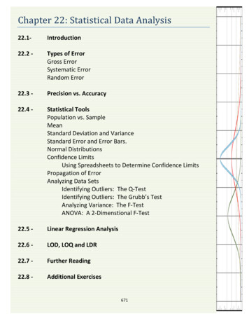
Exercise 22.4: In your own words, explain how changing N and changing σ affects thehistogram generated in the above Activity.A normal probability function represents the way data isscattered about a mean when the error in the sampling isthe result of random error. Figure 22.9 shows a normalprobability distribution with the area under the curveintegrated as a function of standard deviation. We seethat 68.2% of all data points fall within a range of σfrom the mean, 95.4% of all data points fall within 2σ ofthe mean and by the time we get to 3σ from the meanwe have incorporated 99.7% of all data points. If werepeated an analysis 1000 times, we could reasonablyexpect that only 3 data points would fall outside the 3σrange. Knowing the standard deviation allows us topredict the likelihood of the next sampled data pointresiding within a specified range from the mean.Figure 22.9:Normal probabilitydistribution. The ranges indicate thepercentage of all data points as afunction of the distance from themean. The x-axis is in standarddeviations from the mean.Example 22.1: The Bell Curve’s shape as a function of the standard deviationFigure 22.10 shows two different normalprobability functions (npf). Imagine these two npfcurves represent the analysis of a chemicalsample under different experimental conditions.Each experiment produced a sample mean of 50however one technique produced a data set witha standard deviation of 5 while the other data sethad a standard deviation of 10. In the case wheres 5, nearly 99.7% of all data points fell withinthe range of 40 – 60. In the case where s 10, wehave to expand the range to 20 – 80 in order tocapture 99.7% of all data points. If we could onlyFigure 22.10: Two npf curves. The narrow curveafford to repeat the analysis a few times (time has a standard deviation of 5. The wide curve has a ) we would have a lot more confidence that ourstandard deviation of 10.sample mean is close to the population mean forthe technique where s 5 than we would for the technique where s 10.681
Activity –Plotting a normal distribution function in Excel Create the following worksheet in Excel (See Figure 22.11)Create a column of numbers from 2 to 600 in intervals of 2in cells A2 A601. Place a mean value of 301 in cell D1and your standard deviation of 50 in cell D2. Then select cellB2 and click the “insert function” link (fx) and chooseNORMDIST. The ”Function Arguments” box will open. Forthe “x” argument choose cell A2. For the “Mean” argumentbox, type D 1 and for the standard deviation argumentbox, type D 2. The dollar signs in the cell addresses lockthe addresses and prevent them from scrolling. In the“Cumulative” argument field type the word “FALSE”. TheNORMTDIST function will use Equation 22.5 to return aprobability value for obtaining a value of “2” in cell B2.Select cell B2 again and drag and drop it to cell B601. The“B” column now contains the probability of obtaining thevalues listed in the “A” column. Plot an XY scatter plot ofcells A2:A601 vs. B2:B601 and insert the graph in yourworksheet. You should see a classic “bell curve”. Now play Figure 22.11: Example Spreadsheet forwith your mean and standard deviation values and observe programing a Gaussian Curve.how the shape of the Gaussian distribution changes as a function of each variable.Confidence LimitsEarlier we learned how to calculate a standard error. Another common statistical tool forreporting the uncertainty (precision) of a measurement is the confidence limit (CL). Forexample we might report the percent alcohol in a solution as 13% with a 95% CL of 2%, wherethe 2% represents the CL.Unless otherwise stated, the reported CL is at the 95% CL and represents the range in which weare 95% certain the “true” answer lies. The reason the 95% CL is the accepted norm is because95.4% of all data points in a normal distribution is encompassed by a range of approximately 2σ. It is reported at 95% instead of 95.4% for purposes of simplicity. However as you willsoon see, it is possible to calculate CL values other than the 95% CL.We define CL using σ. Recall that σ is the standard deviation of the entire population. Whenwe do not know σ we use “s” instead and a fudge factor, which we will describe shortly. If weknow the standard deviation for the entire population, then the 95% CL 10 is simply95% CL 2σEq. 22.7and we would report the mean as10To be completely accurate, the 95% confidence limit is actually the 95.4% confidence limit because it represents 2σ from the mean (see Figure 22.5).682
µ 2σHowever we seldom know the mean or the standard deviation of an entire population. Allchemical analyses deals with a sampled populations. The CL for a sample is given in ��𝑪𝑪𝑪𝑪𝑪𝑪𝑪𝑪𝑪𝑪 𝒍𝒍𝒍𝒍𝒍𝒍𝒍𝒍𝒍𝒍 𝒕𝒕and we would report the average as11 𝒕𝒕𝒙𝒙𝒔𝒔 𝑵𝑵𝒔𝒔 𝑵𝑵 is the mean of the sample, “s” is thewere 𝒙𝒙standard deviation of the sample, N is the number ofdata points in the sample and “t” is a “fudge factor”taken from Table 22.1.Using Spreadsheets to Determine Confidence LimitsAs we have seen, modern spreadsheets such asMicrosoft Excel are capable of very sophisticatedstatistical analysis. The following Activity will walkyou through the steps of calculating the CL for asample mean.Activity- Using Excel to calculate confidence limits.Open the spreadsheet Fish that you created in theprevious activities. We are going to use Excel todetermine the 95% CL of our data set.Select cell B16 and click on the fx button once again.From the Insert Function dialog box selectCONFIDENCE.NORM. The following dialog box willappear. To calculate a 95% CL you need to input the1112Recall that we defined𝒔𝒔 𝑵𝑵as the standard error in Equation 22.5.The term (N-1) is the degrees of freedom for the sample set.683Eq. 22.8Table 22.1: Confidence Limit t-values as afunction of (N-1) 12N-1 90%95%99%99.5%22.920 4.3039.925 14.08932.353 3.1825.841 7.45342.132 2.7764.604 5.59852.015 2.5714.032 4.77361.943 2.4473.707 4.31771.895 2.3653.500 4.02981.860 2.3063.355 3.83291.833 2.2623.205 3.690101.812 2.2283.169 3.581
uncertainty in the Alpha field as 1.00 – CL You needto input the CL as a decimal (1.00 – 0.95 0.05).Enter the standard deviation (or the address of thestandard deviation) into the “Standard dev” field. Inthe “Size” field enter the value of “N”; the totalnumber of data points (10) and click “OK”.At this point, your spreadsheet should resem
Figure 22.1: Three targets. Target (a) has relatively high accuracy but relatively low precision. Target (b) has relatively low accuracy but relatively high precision. Target (c) has relatively high accuracy and relatively high precision. preparing the sample for analysis. For exait is common to esterify carboxylic acids prior mple,