Transcription
11. Perturbation Theory11.1 Time-independent perturbation theory11.1.1 Non-degenerate case11.1.2 Degenerate case11.1.3 The Stark effect11.2 Time-dependent perturbation theory11.2.1 Review of interaction picture11.2.2 Dyson series11.2.3 Fermi’s Golden Rule11.1 Time-independent perturbation theoryBecause of the complexity of many physical problems, very few can be solved exactly (unless they involve onlysmall Hilbert spaces). In particular, to analyze the interaction of radiation with matter we will need to developapproximation methods36 .11.1.1 Non-degenerate caseWe have an HamiltonianH H0 ǫVwhere we know the eigenvalue of the unperturbed Hamiltonian H0 and we want to solve for the perturbed caseH H0 ǫV , in terms of an expansion in ǫ (with ǫ varying between 0 and 1). The solution for ǫ 1 is the desiredsolution.We assume that we know exactly the energy eigenkets and eigenvalues of H0 :(0)H0 k) Ek k)LAs H0 is hermitian, its eigenkets form a complete basis k k)(k 11. We assume at first that the energy spectrum(0)is not degenerate (that is, all the Ek are different, in the next section we will study the degenerate case). Theeigensystem for the total hamiltonian is then(H0 ǫV ) ϕk )ǫ Ek (ǫ) ϕk )ǫwhere ǫ 1 is the case we are interested in, but we will solve for a general ǫ as a perturbation in this parameter:)))(0)(1)(2)(0)(1)(2) ϕk ) ϕk ǫ ϕk ǫ2 ϕk . . . , Ek Ek ǫEk ǫ2 Ek . . .36A very good treatment of perturbation theory is in Sakurai’s book –J.J. Sakurai “Modern Quantum Mechanics”, Addison Wesley (1994), which we follow here.107
(0)where of course ϕk)(0) k). When ǫ is small, we can in fact approximate the total energy Ek by Ek . The energy(0)shift due to the perturbation is then only k Ek Ekand we can write:(0)(0)(H0 ǫV ) ϕk ) (Ek k ) ϕk )ǫ (Ek H0 ) ϕk ) (ǫV k ) ϕk )Then, we project onto (k :(0)(k (Ek H0 ) ϕk ) (k (ǫV k ) ϕk )(0)The LHS is zero since (k H0 ϕk ) (k Ek ϕk ), and from the RHS (k (ǫV k ) ϕk ) 0 we obtain: k ǫ(k V ϕk )(k ϕk ) k ǫ(k V ϕk )where we set (k ϕk ) 1 (a non-canonical normalization, although, as we will see, it is approximately valid).Using the expansion above, we can replace k by ǫEk1 ǫ2 Ek2 . . . and ϕk ) by its expansion:))(1)(2)ǫEk1 ǫ2 Ek2 · · · ǫ (k V ( k) ǫ ϕk ǫ2 ϕk . . . )and equating terms of the same order in ǫ we obtain:(n 1)Ekn (k V ϕk)This is a recipe to find the energy at all orders based only) on the knowledge of the eigenstates of lower orders.(n 1)However, the question still remains: how do we find ϕk?We could think of solving the equation:(0)(Ek H0 ) ϕk ) (ǫV k ) ϕk )( )(0)for ϕk ), by inverting the operator (Ek H0 ) and again doing an expansion of ϕk ) to equate terms of the sameorder:))(1)(0)(1) k) ǫ ϕk · · · (Ek H0 ) 1 (ǫV k )( k) ǫ ϕk . . . )(0)Unfortunately this promising approach is not correct, since the operator (Ek H0 ) 1 is not always well defined.(0)(0)Specifically, there is a singularity for (Ek H0 ) 1 k). What we need is to make sure that (Ek H0 ) 1 is neverapplied to eigenstates of the unperturbed Hamiltonian,that is, we need ψk ) (ǫV k ) ϕk ) 6 k) for any ϕk ).LWe thus define the projector Pk 11 k) (k h k h)(h .Thenwecanensurethat ψ)the projected state6 ψ)′ Pk ψ) is such that (k ψ ′ ) 0 since this is equal to(k Pk ψ) (k ψ) (k k)(k ψ) 0(0)Now, using the projector, (Ek H0 ) 1 Pk ψ) is well defined. We then take the equation ( ) and multiply it by Pkfrom the left:(0)Pk (Ek H0 ) ϕk ) Pk (ǫV k ) ϕk ) .(0)(0)Since Pk commutes with H0 (as k) is an eigenstate of H0 ) we have Pk (Ek H0 ) ϕk ) (Ek H0 )Pk ϕk ) and wecan rewrite the equation as(0)Pk ϕk ) (Ek H0 ) 1 Pk (ǫV k ) ϕk )We can further simplify this expression, noting that Pk ϕk ) ϕk ) k)(k ϕk ) ϕk ) k) (since we adopted thenormalization (k ϕk ) 1). Finally we obtain:(0) ϕk ) k) (Ek H0 ) 1 Pk (ǫV k ) ϕk )108( )
This equation is now ready to be solved by using the perturbation expansion. To simplify the expression, we definethe operator RkL h) (h (0)Rk (Ek H0 ) 1 Pk Ek0 Eh06h kNow using the expansion(1)(1) k) ǫ ϕk ) · · · k) Rk ǫ(V Ek1 ǫEk2 . . . )( k) ǫ ϕk ) . . . )we can solve term by term to obtain:1st order:(1) ϕk ) Rk (V Ek1 ) k) Rk (V (k V k)) k) Rk V k)(where we used the expression for the first order energy and the fact that Rk k) 0 by definition).We can now calculate the second order energy, since we know the first order eigenstate: L h) (h (1)Ek2 (k V ϕk ) (k V Rk V k) (k V V k)Ek0 Eh06h kor explicitlyEk2 L Vkh 2Ek0 Eh06h kThen the second order eigenstate is2nd order:ϕ2k Rk V Rk V k)A. Formal SolutionWe can also find a more formal expression that can yield the solution to all orders. We rewrite Eq. (**) using Rkand obtain ϕk ) k) Rk (ǫV k ) ϕk ) Rk H1 ϕk )where we defined H1 (ǫV k ). Then by iteration we can write:and in general: ϕk ) k) Rk H1 ( k) Rk H1 ϕk )) k) Rk H1 k) Rk H1 Rk H1 ϕk ) ϕk ) k) Rk H1 k) Rk H1 Rk H1 k) · · · (Rk H1 )n k) . . .This is just a geometric series, with formal solution: ϕk ) (11 Rk H1 ) 1 k)B. NormalizationIn deriving the TIPT we introduced a non-canonical normalization (k ϕk ) 1, which implies that the perturbedstate ϕk ) is not normalized. We can then define a properly normalized state as ψk ) v ϕk )(ϕk ϕk )vso that (k ψk ) 1/ (ϕk ϕk ). We can calculate perturbatively the normalization factor (ϕk ϕk ):L Vkh 2121 12 (ϕk ϕk ) (k ǫϕ1k . . . k ǫϕ1 . . .) 1 ǫ(k ϕ0 k ) . ǫ (ϕk ϕk ) . 1 ǫ(E E 0 )26h kNotice that the state is correctly normalized up to the second order in ǫ.109hk
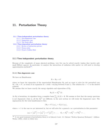
C. Anti-crossingConsider two levels, h and k with energies Ek0 and Eh0 and assume that we apply a perturbation V which connectsonly these two states (that is, V is such that (l V j) 0 and it is different than zero only for the transition from hto k: (h V k) 6 0.)If the perturbation is small, we can ask what are the perturbed state energies.The first order is zero by the choice of V , then we can calculate the second order:(2)Ek L Vkj 2 Vkh 2 Ek0 Ej0Ek0 Eh06j kand similarly(2)Eh L Vhj 2 Vkh 2(2) 0 Ek .00Eh EjEh Ek06j hThis opposite energy shift will be more important (more noticeable) when the energies of the two levels Ek0 andEh0 are close to each other. Indeed, in the absence of the perturbation, the two energy levels would “cross” whenEk0 Eh0 . If we add the perturbation, however, the two levels are repelled with opposite energy shifts. We describewhat is happening as an “anti-crossing” of the levels: even as the levels become connected by an interaction, the levelsnever meet (never have the same energy) since each level gets shifted by the same amount in opposite directions.D. Example: TLS energy splitting from perturbationConsider the Hamiltonian H ωσz ǫΩσx . For ǫ 0 the eigenstates are k) { 0), 1)} and eigenvalues Ek0 ω.We also know how to solve exactly this simple problem by diagonalizing the entire matrix:vE1,2 ω 2 ǫ2 Ω 2 , ϕ1 ) cos(ϑ/2) 0) sin(ϑ/2) 1), ϕ2 ) cos(ϑ/2) 1) sin(ϑ/2) 0) withϑ arctan(ǫΩ/ω)For ǫ 1 we can expand in series these results to find:E1,2 (ω ǫ2 Ω 2 .)2ωϑǫΩϑǫΩ 1) 0) 1) ϕ2 ) 1) 0) 1) 0)22ω22ωAs an exercise, we can find as well the results of TIPT. First we find that the first order energy shift is zero, sinceEk1 (k V k) (0 (Ωσx ) 0) 0 (and same for (1 (Ωσx ) 1)). Then we can calculate the first order eigenstate: ϕ1 ) 0) ϕ11 0) (E10 H0 ) 1 P1 V 0) 0) [ω(11 σz )] 1 1)(1 ǫΩσx 0) 0) 1ΩǫΩ 1)(1 σx 0) 0) ǫ 1)2ω2ω22 (ǫΩ)Ωsimilarly, we find ϕ12 1) ǫ 2ω 0). Finally, the second order energy shift is E12 E V0 12in agreement0 2ω1 E2with the result from the series expansion.We can also look at the level anti-crossing: If we vary the energy ω around zero, the two energy levels cross eachother.110
EigenvaluesΩFig. 18: Level anticrossing: Eigenvalues of the Hamiltonian H ωσz ǫΩσx as a function of ω. Dashed lines: Ω 0. Redlines: Ω 0 showing the anticrossing.11.1.2 Degenerate caseIf there are degenerate (or quasi-degenerate) eigenvalues of the unperturbed Hamiltonian H0 , the expansion usedabove is no longer valid. There are two problems:1. If k ′ ), k ′′ ), . have the same eigenvalue, we can choose any combination of them as the unperturbed eigenket.But then, if we were to find the perturbed eigenket ψk ), to which state would this go to when ǫ 0?can be singular for the degenerate eigenvalues.2. The term Rk (0)PkEk H0Assume there is a d-fold degeneracy of the eigenvalueEd , with the unperturbed eigenkets { ki )} forming a subspaceLHd . We can then define the projectors Qd ki Hd ki )(ki and Pd 11 Qd. These projectors also define subspacesof the total Hilbert space H that we will call Hd (spanned by Qd ) and Hd̄ (spanned by Pd ).Notice that because of their nature of projectors, we have the following identities:Pd2 Pd ,Q2d Qd ,Pd Qd Qd Pd 0andPd Qd 11.We then rewrite the eigenvalue equation as:(H0 ǫV ) ϕk ) Ek ϕk ) H0 (Qd Pd ) ϕk ) ǫV (Qd Pd ) ϕk ) Ek (Qd Pd ) ϕk ) (Qd Pd )H0 ϕk ) ǫV (Qd Pd ) ϕk ) Ek (Qd Pd ) ϕk )where we used the fact that [H0 , Qd ] [H0 , Pd ] 0 since the projectors are diagonal in the Hamiltonian basis. Wethen multiply from the left by Qd and Pd , obtaining 2 equations:1.Pd [(Qd Pd )H0 ϕk ) ǫV (Qd Pd ) ϕk )] Pd (Ek (Qd Pd ) ϕk )) 2.H0 Pd ϕk ) ǫPd V (Qd Pd ) ϕk ) Ek Pd ϕk )Qd [(Qd Pd )H0 ϕk ) ǫV (Qd Pd ) ϕk )] Qd (Ek (Qd Pd ) ϕk )) H0 Qd ϕk ) ǫQd V (Qd Pd ) ϕk ) Ek Qd ϕk )and we simplify the notation by setting ψk ) Pd ϕk ) and χk ) Qd ϕk )H0 ψk ) ǫPd V ( χk ) ψk )) Ek ψk )H0 χk ) ǫQd V ( χk ) ψk )) Ek χk )111
which gives a set of coupled equations in ψk ) and χk ): 1Now (Ek H0 ǫPd V Pd )1.ǫPd V χk ) (Ek H0 ǫPd V Pd ) ψk )2.ǫQd V ψk ) (Ek H0 ǫQd V Qd ) χk )is finally well defined in the Pd subspace, so that we can solve for ψk ) from (1.): ψk ) ǫPd (Ek H0 ǫPd V Pd ) 1 Pd V χk )and by inserting this in (2.) we find(Ek H0 ǫQd V Qd ) χk ) ǫ2 Qd V Pd (Ek H0 ǫPd V Pd ) 1 Pd V χk ) .If we keep only the first order in ǫ in this equation we have:[(Ek Ed ) ǫQd V Qd ] χk ) 0which is an equation defined on the subspace Hd only.We now call Ud Qd V Qd the perturbation Hamiltonian in the Hd space and k (Ek Ed )11d , to get:( k ǫUd ) χk ) 0Often it is possible to just diagonalize Ud (if the degenerate subspace is small enough, for example for a simple doubledegeneracy) and notice that of course k is already diagonal. Otherwise one can apply perturbationtheoryto this)))(0)(0)(0)subspace. Then we will have found some (exact or approximate) eigenstates of Ud , ki , s.t. Ud ki ui ki))(0)(0)and H0 ki Ed ki , i. Thus, this step sets what unperturbed eigenstates we should choose in the degeneratesubspace, hence solving the first issue of degenerate perturbation theory.We now want to look at terms ǫ2 in 1 Pd V χk )(Ek H0 ǫUd ) χk ) ǫ2 Qd V Pd (Ek H0 ǫP d V Pd )where we neglected terms higher than second order. Rearranging the terms, we have:Ek χk ) [H0 ǫUd ǫ2 Qd V Pd (Ek H0 ) 1 Pd V ] χk )with (H̃0 Ṽ ) χk ) Ek χk )Ṽ ǫQd V Pd (Ek H0 ) 1 Pd V QdH̃0 H0 ǫUd(n)If there are no degeneracies left in H̃0 , we can solve this problem by TIPT and find χkFor example, to first order, we have))) L kj(0) V ki(0)(1)(0)χk,i kjǫ(ui uj )).6j i(0)(0)and using the explicit form of the matrix element Ṽij (kj Ṽ ki ),(0)Ṽij kj(0)ǫ2 V Pd (Ed0 H0 ) 1 Pd V kiwe obtain:(1)χk,i)) ǫ2Lh H/ d(0)kj(0)V h) (h V kiL (kj(0) V h) (h V k (0) ) (0) )i ǫk(ui uj ) E (0) E (0) jj i6d112h(0)(0)Ed Eh)
Finally, we need to add χ) and ψ) to find the total vector:D) (0)(0)))(h VkV h)kLLji(1)(0) (h V ki ) h) ǫ kjϕk(0)(0)(0)0(u u)ijE EE E6j idhdhh H/ d(1)ϕk) L (kj(0) V h) (0) )L (h V ki ) h) ǫ k(0)0(ui uj ) j6j ih H/ d Ed EhExample: Degenerate TLSConsider the Hamiltonian H ωσz ǫΩσx . We already solved this Hamiltonian, both directly and with TIPT.Now consider the case ω 0 and a slightly modified Hamiltonian:H (ω0 ω) 0)(0 (ω0 ω) 1)(1 ǫΩσx ω0 11 ωσz ǫΩσx .We could solve exactly the system for ω 0, simply finding E0,1 ω0 ǫΩ and ϕ)0,1 ) 12 ( 0) 1)). Wecan also apply TIPT.However the two eigenstates 0), 1) are (quasi-)degenerate thus we need to apply degenerate perturbation theory. Inparticular, any basis arising from a rotation of these two basis states could be a priori a good basis, so we need firstto obtain the correct zeroth order eigenvectors. In this very simple case we have Hd H (the total Hilbert space)and Hd 0, or in other words, Qd 11, Pd 0. We first need to define an equation in the degenerate subspace only:( k ǫUd ) χk ) 0where Ud Qd V Qd . Here we have: Ud V Ωσx . Thus we obtain the correct zeroth order eigenvectors fromdiagonalizing this Hamiltonian. Not surprisingly, they are:)1(0)ϕ0,1 ) ( 0) 1)).2with eigenvalues: E0,1 ω0 ǫΩ. We can now consider higher orders, from the equation: 0 Ṽ ) χk ) Ek χk )(Hwith H̃0 ω0 11 ǫΩσx and Ṽ 0. Thus in this case, there are no higher orders and we solved the problem.Example: Spin-1 systemWe consider a spin-1 system (that is, a spin system with S 1 defined in a 3-dimensional Hilbert space). The matrixrepresentation for the angular momentum operators Sx and Sz in this Hilbert space are: 1 0 01 0 1 0 1 0 1Sx , Sz 0 0 0 20 1 00 0 1The Hamiltonian of the system is H H0 ǫV withH0 Sz2 ;Given thatV S x Sz 1 0Sz2 0 00 0113 00 1
The matrix representation of the total Hamiltonian is : ǫǫH 20 ǫ20 ǫ20 ǫ2 ǫ Possible eigenstates of the unperturbed Hamiltonian are 1) , 0), 1): 100 1) 0 , 0) 1 , 1) 0 ,001with energies , 0, respectively. However, any combination of 1)we could have chosen: 111 1) 0 , 1) 221and 1) is a valid eigenstate, for example 10 1This is the case because the two eigenstates are degenerate. So how do we choose which are the correct eigenstatesto zeroth order37 ? We need to first consider the total Hamiltonian in the degenerate subspace.The degenerate subspace is the subspace of the total Hilbert space H spanned by the basis 1) , 1); we can callthis subspace HQ . We can obtain the Hamiltonian in this subspace by using the projector operator Q: HQ QHQ,with Q 1)( 1 1)( 1 Sz2 . Then:HQ Q( Sz2 ǫ(Sz Sx ))Q Sz2 ǫSz(Notice this can be obtained by direct matrix multiplication or multiplying the operators). In matrix form: () ǫ 00 ǫ000 HQ HQ 00 ǫ00 ǫwhere in the last line I represented the matrix in the 2-dimensional subpsace HQ . We can now easily see that thecorrect eigenvectors for the unperturbed Hamiltonian were the original 1) and 1) after all. From the Hamiltonianin the HQ subspace we can also calculate the first order correction to the energy for the states in the degenerate(1)(0)(1)(0)subspace. These are just E 1 E 1 ǫ and E 1 E 1 ǫ.(1)Now we want to calculate the first order correction to the eigenstates 1). This will have two contributions: ψ) 1 (1)(1)Q ψ) 1 P ψ) 1 where P 11 Q 0) (0 is the complementary projector to Q. We first calculate the first termin the following way. We redefine an unperturbed Hamiltonian in the subspace HQ :H̃0 HQ QHQ Sz2 ǫSzand the perturbation in the same subspace is (following Sakurai): ǫṼ VQ ǫQ(V P ( H0 ) 1 P V )Q ǫQ (Sz Sx ) 0) (0 ( 0) (0 ) 1 0) (0 (Sz Sx ) Q QSx P Sx Q In matrix form: ǫ 1 00 0VQ 2 1 0 ()1ǫǫ1 1 0 (11 σx ) VQ 1 12 2 1Now the perturbed eigenstates can be calculated as:(1)Q ψ)k k) ǫLh HQ k37(h VQ k)(1)(1)Ek Eh h)Here by correct eigenstates I means the eigenstates to which the eigenstates of the total Hamiltonian will tend to whenǫ 0114
In our case:(1)Q ψ) 1 1) ǫ( 1 VQ 1)(1)E 1 (1)E 1 1) 1) ǫǫ ( 1 (11 σx ) 1)ǫ 1) 1) 1) ,2 2ǫ4 (1)Qψ 1 1) ǫ 1)4 (1)In order to calculate P ψ 1 we can just use the usual formula for non-degenerate perturbation theory, but summingonly over the states outside HQ . Here there’s only one of them 0), so :(1)P ψ) 1 ǫǫ(0 V 1) 0) 0)E 1 E02 Finally, the eigenstates to first order are: ψ 1 )and(1) 1) (1) ψ 1 )ǫǫ 1) 0)4 2 ǫǫ 1) 0)4 2 L (h V 1) 2 :(0) Ehh H/ Q 1) (2)The energy shift to second order is calculated from (2) 1 ǫ2 (0 V 1) 2 2 andǫ2 (0 V 1) 2 2 To calculate the perturbation expansion for 0) and its energy, we use non-degenerate perturbation theory, to find:(2) 1 (1) ψ 1 )(2)2(1) 0) ǫ( 1 (0 V 0) 0)( 1 V 0)( 1 V 0)ǫ 1) 1) 1) 1) 2and 0 ǫ .11.1.3 The Stark effectWe analyze the interaction of a hydrogen atom with a (classical) electric field, treated as a perturbation38 . Dependingon the hydrogen’s state, we will need to use TIPT or degenerate TIPT, to find either a quadratic or linear (in thefield) shift of the energy. The shift in energy is usually called Stark shift or Stark effect and it is the electric analogueof the Zeeman effect, where the energy level is split into several components due to the presence of a magnetic field.Measurements of the Stark effect under high field strengths confirmed the correctness of the quantum theory overthe Bohr model.Suppose that a hydrogen atom is subject to a uniform external electric field, of magnitude E , directed along thez-axis. The Hamiltonian of the system can be split into two parts. Namely, the unperturbed Hamiltonian,H0 38p2e2 ,2 me 4π ǫ0 rThis section follows Prof. Fitzpatrick online lectures115
and the perturbing HamiltonianH1 e E z.Note that the electron spin is irrelevant to this problem (since the spin operators all commute with H1 ), so we canignore the spin degrees of freedom of the system. Hence, the energy eigenstates of the unperturbed Hamiltonian arecharacterized by three quantum numbers–the radial quantum number n, and the two angular quantum numbers land m. Let us denote these states as the nlm), and let their corresponding energy eigenvalues be the Enlm . We useTIPT to calculate the energy shift to first and second order.A. The quadratic Stark effectWe first want to study the problem using non-degenerate perturbation theory, thus assuming that the unperturbedstates are non-degenerate. According to TIPT, the change in energy of the eigenstate characterized by the quantumnumbers n, l, m in the presence of a small electric field is given by Enlm e E (n, l, m z n, l, m) e2 E 2Ln′ ,l′ ,m′ n,l,m (n, l, m z n′ , l′ , m′ ) 2.Enlm En′ l′ m′This energy-shift is known as the Stark effect. The sum on the right-hand side of the above equation seems verycomplicated. However, it turns out that most of the terms in this sum are zero. This follows because the matrixelements (n, l, m z n′ , l′ , m′ ) are zero for virtually all choices of the two sets of quantum number n, l, m and n′ , l′ , m′ .Let us try to find a set of rules which determine when these matrix elements are non-zero. These rules are usuallyreferred to as the selection rules for the problem in hand.Now, since [Lz , z] 0, it follows that(n, l, m [Lz , z] n′ , l′ , m′ ) (n, l, m Lz z z Lz n′ , l′ , m′ ) l (m m′ ) (n, l, m z n′ , l′ , m′ ) 0.Hence, one of the selection rules is that the matrix element (n, l, m z n′ , l′ , m′ ) is zero unlessm′ m.The selection rule for l can be similarly calculated from properties of the total angular momentum L2 and itscommutator with z. We obtain that the matrix element is zero unlessl′ l 1.Application of these selection rules to the perturbation equation shows that the linear (first order) term is zero, whilethe second order term yieldsL (n, l, m z n′ , l′ , m) 2 Enlm e2 E 2.Enlm En′ l′ m′ ′n ,l l 1Only those terms which vary quadratically with the field-strength have survived. Hence, this type of energy-shift ofan atomic state in the presence of a small electric field is known as the quadratic Stark effect.Now, the electric polarizability of an atom is defined in terms of the energy-shift of the atomic state as follows:1 E α E 2 .2Hence, we can writeαnlm 2 e2Ln′ ,l′ l 1 (n, l, m z n′ , l′ , m) 2.En′ l′ m EnlmAlthough written for a general state, the equations above assume there is no degeneracy of the unperturbed eigen values. However, the unperturbed eigenstates of a hydrogen atom have energies which only depend on the radialquantum number n, thus they have high (and increasing with n) order of degeneracy. We can then only apply theabove results to the n 1 eigenstate (since for n 1 there will be coupling to degenerate eigenstates with the same116
value of n but different values of l). Thus, according to non-degenerate perturbation theory, the polarizability of theground-state (i.e., n 1) of a hydrogen atom is given byα 2 e2L (1, 0, 0 z n, 1, 0) 2.En E1n 1Here, we have made use of the fact that En10 En00 En .The sum in the above expression can be evaluated approximately by noting thatEn where a0 4π ǫ0 2me e2e2,8π ǫ0 a0 n2is the Bohr radius. Hence, we can writeEn E1 E2 E1 3e2,4 8π ǫ0 a0which implies that the polarizability isα L16 (1, 0, 0 z n, 1, 0) 2.4π ǫ0 a03n 1LHowever, thanks to the selection rules we have, n 1 (1, 0, 0 z n, 1, 0) 2 (1, 0, 0 z 2 1, 0, 0) 13 (1, 0, 0 r2 1, 0, 0),where we have made use of the fact the the ground-state of hydrogen is spherically symmetric. Finally, from(1, 0, 0 r2 1, 0, 0) 3 a02 we conclude thatα 164π ǫ0 a03 5.3 4π ǫ0 a03 .3The exact result (which can be obtained by solving Schrdinger’s equation in parabolic coordinates) isα 94π ǫ0 a03 4.5 4π ǫ0 a03 .2B. The linear Stark effectWe now examine the effect of an electric field on the excited energy levels n 1 of a hydrogen atom. For instance,consider the n 2 states. There is a single l 0 state, usually referred to as 2s, and three l 1 states (withm 1, 0, 1 ), usually referred to as 2p. All of these states possess the same energy, E2 e2 /(32πǫ0 a0 ). Becauseof the degeneracy, the treatment above is no longer valid and in order to apply perturbation theory, we have to recurto degenerate perturbation theory.We first need to Ud Qd V Qd , where Qd is the projector obtained from the degenerate 2s and 2p states (that is, theoperator that project into the degenerate subspace). This operator is, 0(2, 0, 0 z 2, 1, 0) 0 0()00 0 0(2, 0, 0 z 2, 1, 0) (2, 1, 0 z 2, 0, 0)Ud e E ,000 0 (2, 1, 0 z 2, 0, 0)0000 0where the rows and columns correspond to the 2, 0, 0), 2, 1, 0), 2, 1, 1) and 2, 1, 1) states, respectively and in thesecond step we reduce the operator to the degenerate subspace only. To simplify the matrix we used the selectionrules, which tell us that the matrix element of between two hydrogen atom states is zero unless the states possess thesame n quantum number, and l quantum numbers which differ by unity. It is easily demonstrated, from the exactforms of the 2s and 2p wave-functions, that(2, 0, 0 z 2, 1, 0) (2, 1, 0 z 2, 0, 0) 3 a0 .117
It can be seen, by inspection, that the eigenvalues of Ud are u1 3 e a0 E , u2 3 e a0 E , with correspondingeigenvectors()) 2, 0, 0) 2, 1, 0)11(0) ,k1122()) 2, 0, 0) 2, 1, 0)11(0) k2 122In the absence of an electric field, all of these states possess the same energy, E2 . The first-order energy shifts inducedby an electric field are given by E1 E2 3 e a0 E , 3 e a0 E ,Thus, the energies of states 1 and 2 are shifted upwards and downwards, respectively, by an amount 3 e a0 E in thepresence of an electric field. States 1 and 2 are orthogonal linear combinations of the original 2s and 2p(m 0) states.Note that the energy shifts are linear in the electric field-strength, so this is a much larger effect that the quadraticeffect described in the previous section.The energies of states 2p(m 1) and 2p(m -1) (which are outside the degenerate subspace) are not affected to first order (as we already saw above for the non-degenerate case). Of course, to second-order the energies of these states areshifted by an amount which depends on the square of the electric field-strength, the quadratic shift found previously.Note that the linear Stark effect depends crucially on the degeneracy of the 2s and 2p states. This degeneracy is aspecial property of a pure Coulomb potential, and, therefore, only applies to a hydrogen atom. Thus, alkali metalatoms do not exhibit the linear Stark effect.118
11.2 Time-dependent perturbation theory11.2.1 Review of interaction pictureWhen first studying the time evolution of QM systems, one approach was to separate the Hamiltonian much in thesame way we did above for TIPT. We wrote (see Section 5.2):H H0 V (t)where H0 is a ”solvable” Hamiltonian of which we already know the eigen-decomposition,H0 k) Ek0 k),(so that it is easy to calculate e.g. U0 e iH0 t ) and V (t) is a perturbation that drives an interestingL(althoughunknown) dynamics. Here we even allow for the possibility that V is time-dependent. For any state ψ) k ck (0) k)L0the evolution can be written as ψ) k ck (t)e iEk t k). This correspond to explicitly writing down the evolution dueto the known Hamiltonian (if H H0 then we would have ck (t) ck (0) and the evolution would be given by only thephase factors). In other words, if we want to compare the state evolution with the initial eigenstates, by calculatingthe overlap (k ψ(t)) 2 , we would be really interested only in the dynamics driven by V since (k ψ(t)) 2 ck (t) 2(while Ek0 do not play a role).We define states in the interaction picture by ψ)I U0 (t)† ψ) eiH0 t ψ)Similarly we define the corresponding interaction picture operators as:AI (t) U0† AU0 VI (t) U0† V U0We can now derive the differential equation governing the evolution of the state in the interaction picture, startingfrom Schrödinger equation. (U0† ψ)) ψ)I U † ψ) i i( 0 ψ) U0†)i t t t tInserting t U0 iH0 U0 and i t ψ) H0 ψ), we obtaini ψ) U0† H0 ψ) U0† (H0 V ) ψ) U0† V ψ). tInserting the identity 11 U0 U0† , we obtain U0† V U0 U0† ψ) VI ψ)I :i ψ)I VI (t) ψ)I tThis is a Schrödinger -like equation for the vector in the interaction picture, evolving under the action of the operatorVI (t) only.11.2.2 Dyson seriesBesides expressing the Schrödinger equation in the interaction picture, we can also write the equation for the prop agator that describes the evolution of the state:d UI iVI UI ,dt ψ(t))I UI (t) ψI (0))119
Since VI (t) is time-dependent, we can only write formal solutions for UI . One expression is given by the Dyson series.The differential equation is equivalent to the integral equation1 tUI (t) 11 iVI (t′ )UI (t′ )dt′0By iterating, we can find a formal solution to this equation :UI (t) 11 i1 ( i)n1t′2dt VI (t ) ( i)00This is the Dyson series.′1tdt′0tdt′ . . .11t′dt′ VI (t′ )VI (t′′ ) . . .0t(n 1)dt(n) VI (t′ ) . . . VI (t(n) ) . . .011.2.3 Fermi’s Golden RuleThe problem that we try to solve via TDPT is to calculate the transition probability from an initial state to a finalstate. Consider an initial state i) which is an eigenstate of H0 (H0 i) Ei i)). Then in the interaction picture wehave the evolutionL i(t))I UI (t) i) ck (t) k), with ck (t) (k UI (t) i)kWe can insert the perturbation expansion for UI (t) to obtain an expansion for ck (t):ck (t) (k 11 i10t′′′VI (t )UI (t )dt i) (k 11 i1t′′2dt VI (t ) ( i)01tdt0′1t′0dt′ VI (t′ )VI (t′′ ) . . . i)In the expansion we will obtain terms such as (k VI (t) i) that we can simplify since:(k VI (t) i) (k (U0† V (t)U0 ) i) (U0 k V (t) U0 i) (k eiωk t V (t)e iωi t i) (k V i) eiωki t Vki (t)eiωki twhere we defined ωj Ej /l and ωki ωk ωi . Using these relationships and the series expansion we obtain:(0)ck (t) (k 11 i) δkiJtJt′(1)ck (t) i 0 (k VI (t′ ) i) dt′ i 0 Vki (t′ )eiωki t dt′′JJ′′′tt(2)ck (t) 0 dt′ 0 dt′′ Vkh (t′ )Vhi (t′′ )eiωkh t eiωhi tFrom this expansion we can calculate the transition probability as P (i k) ck (t) 2 .We first consider the case where the perturbation V is time-independent and it is turned on at the time t 0. Thenwe have)(1 t′Vki iωki t/2ωki tVki(1)ck (t) iVkieiωki t dt′ (1 eiωki t ) 2iesinωkiωki20Then to first order perturbation, the transition probability is4 Vki 2P (i k) sin22ωki(ωki t2)We can plot this transition probability as a function of the energy separation ωki between the two states. We wouldexpect that if the separation in energy is smaller, it will be easier to make the transition. This is indeed the case,since P has the shape of a sinc function square.Notice that the peak height is proportional to t2 , while the zeros appear at 2kπ/t, that is, the peak width isproportional to 1/t (the other peaks are quite small). This means that the probability is significantly different than120
0.250.200.150.100.05 6 42 246Fig. 19: Transition probabilityzero only for ωki t 2π. In terms of energy, we have that t E l (where we defined t as the duration of theinteraction), or in other words, we can have a change of energy in the system only at short times, while at long timeswe require quasi-conservation of energy. Consider the limit of the sinc function:limt sin(ωt/2) πδ(ω)ωThen, from f (x)δ(x) f (0) and sinc(0) 1, we obtainlimt (sin(ωt/2)ω)2 sin(ωt/2)sin(ωt/2)sin(ωt/2)lim πδ(ω) t ωωω(sin(ωt/2)ωt/2)tπtπδ(ω) δ(ω)22We have then found the transition probability at long time:t P (i k) πtδ(ω) 4 Vki 2 ,2which confirms the fact that in the lo
theory . Because of the complexity of many physical problems, very few can be solved exactly (unless they involve only small Hilbert spaces). In particular, to analyze the interaction of radiation with matter we will need to develop approximation methods.