WIXLIB

Decision TreesMIT 15.097 Course NotesCynthia RudinCredit: Russell & Norvig, Mitchell, Kohavi & Quinlan, Carter, Vanden BerghenWhy trees? interpretable/intuitive, popular in medical applications because they mimicthe way a doctor thinks model discrete outcomes nicely can be very powerful, can be as complex as you need them C4.5 and CART - from “top 10” - decision trees are very popularSome real examples (from Russell & Norvig, Mitchell) BP’s GasOIL system for separating gas and oil on offshore platforms - decision trees replaced a hand-designed rules system with 2500 rules. C4.5-basedsystem outperformed human experts and saved BP millions. (1986) learning to fly a Cessna on a flight simulator by watching human expertsfly the simulator (1992) can also learn to play tennis, analyze C-section risk, etc.How to build a decision tree: Start at the top of the tree. Grow it by “splitting” attributes one by one. To determine which attributeto split, look at “node impurity.” Assign leaf nodes the majority vote in the leaf. When we get to the bottom, prune the tree to prevent overfittingWhy is this a good way to build a tree?1

I have to warn you that C4.5 and CART are not elegant by any means that Ican define elegant. But the resulting trees can be very elegant. Plus there are2 of the top 10 algorithms in data mining that are decision tree algorithms! Soit’s worth it for us to know what’s under the hood. even though, well. let’sjust say it ain’t pretty.Example: Will the customer wait for a table?(from Russell & Norvig)Here are the attributes:1.Alternate: whether there is a suitable alternative restaurant nearby.2.Bar: whether the restaurant has a comfortable bar area to wait in.3.Fri/Sat: true on Fridays and Saturdays.4.Hungry: whether we are hungry.5.Patrons: how many people are in the restaurant (values are None, Some, and Full).6.Price: the restaurant's price range ( , , ).7.Raining: whether it is raining outside.8.Reservation: whether we made a reservation.9.Type: the kind of restaurant (French, Italian, Thai or Burger).10.WaitEstimate: the wait estimated by the host (0-10 minutes, 10-30, 30-60, 60).Image by MIT OpenCourseWare, adapted from Russell and Norvig, Artificial Intelligence:A Modern Approach, Prentice Hall, 2009.Here are the RainResTypeEstWillWaitX1YesNoNoYesSome NoYesFrench0-10YesX2YesNoNoYesFull NoNoThai30-60NoX3NoYesNoNoSome NoNoBurger0-10YesX4YesNoYesYesFull NoNoThai10-30YesX5YesNoYesNoFull NoYesFrench 60NoX6NoYesNoYesSome YesYesItalian0-10YesX7NoYesNoNoNone YesNoBurger0-10NoX8NoNoNoYesSome YesYesThai0-10YesX9NoYesYesNoFull YesNoBurger 60NoX10YesYesYesYesFull NoYesItalian10-30NoX11NoNoNoNoNone NoNoThai0-10NoX12YesYesYesYes NoNo30-60YesFullBurgerImage by MIT OpenCourseWare, adapted from Russell and Norvig, Artificial Intelligence:A Modern Approach, Prentice Hall, 2009.Here are two options for the first feature to split at the top of the tree. Whichone should we choose? Which one gives me the most information?2

X1,X3,X4,X6,X8,X12X2,X5,X7,X9,X10,X11 :-:(a)Patrons?NoneSome :- : X7,X11 : X4,X12- : X2,X5,X9,X10 : X1,X3,X6,X8-:X1,X3,X4,X6,X8,X12X2,X5,X7,X9,X10,X11 :-:Type?(b)French :-:FullItalian : X6- : X10X1X5BurgerThai : X4,X8 : X3,X12- : X2,X11 - : X7,X9Image by MIT OpenCourseWare, adapted from Russell and Norvig,Artificial Intelligence: A Modern Approach, Prentice Hall, 2009.What we need is a formula to compute “information.” Before we do that, here’sanother example. Let’s say we pick one of them (Patrons). Maybe then we’llpick Hungry next, because it has a lot of “information”: ?None :- : X7,X11YesSomeFull : X1,X3,X6,X8-: : X4,X12- : X2,X5,X9,X10NoHungry?YesNo : X4,X12 :- : X2,X10 - :X5,X9Image by MIT OpenCourseWare, adapted from Russell and Norvig,Artificial Intelligence: A Modern Approach, Prentice Hall, 2009.We’ll build up to the derivation of C4.5. Origins: Hunt 1962, ID3 of Quinlan1979 (600 lines of Pascal), C4 (Quinlan 1987). C4.5 is 9000 lines of C (Quinlan1993). We start with some basic information theory.3

Information Theory (from slides of Tom Carter, June 2011)“Information” from observing the occurrence of an event: #bits needed to encode the probability of the event p log2 p.E.g., a coin flip from a fair coin contains 1 bit of information. If the event hasprobability 1, we get no information from the occurrence of the event.Where did this definition of information come from? Turns out it’s pretty cool.We want to define I so that it obeys all these things: I(p) 0, I(1) 0; the information of any event is non-negative, no information from events with prob 1 I(p1 · p2 ) I(p1 ) I(p2 ); the information from two independent eventsshould be the sum of their informations I(p) is continuous, slight changes in probability correspond to slight changesin informationTogether these lead to:I(p2 ) 2I(p) or generally I(pn ) nI(p),this means that I(p) I (p1/m m) mI p1/m 11/mso I(p) I pmand more generally,nI(p).mThis is true for any fraction n/m, which includes rationals, so just define it forall positive reals:I(pa ) aI(p). I pn/m The functions that do this are I(p) logb (p) for some b. Choose b 2 for“bits.”4

Flipping a fair coin gives log2 (1/2) 1 bit of information if it comes up eitherheads or tails.A biased coin landing on heads with p .99 gives log2 (.99) .0145 bits ofinformation.A biased coin landing on heads with p .01 gives log2 (.01) 6.643 bits ofinformation.Now, if we had lots of events, what’s the mean information of those events?Assume the events v1 , ., vJ occur with probabilities p1 , ., pJ , where [p1 , ., pJ ]is a discrete probability distribution.Ep [p1 ,.,pJ ] I(p) JXpj I(pj ) j 1Xpj log2 pj : H(p)jwhere p is the vector [p1 , ., pJ ]. H(p) is called the entropy of discrete distribution p.So if there are only 2 events (binary), with probabilities p [p, 1 p],H(p) p log2 (p) (1 p) log2 (1 p).If the probabilities were [1/2, 1/2],11H(p) 2 log2 1 (Yes, we knew that.)22Or if the probabilities were [0.99, 0.01],H(p) 0.08 bits.As one of the probabilities in the vector p goes to 1, H(p) 0, which is whatwe want.Back to C4.5, which uses Information Gain as the splitting criteria.5

Back to C4.5 (source material: Russell & Norvig, Mitchell, Quinlan)We consider a “test” split on attribute A at a branch.In S we have #pos positives and #neg negatives. For each branch j, we have#posj positives and #negj negatives.The training probabilities in branch j are: #posj#negj,.#posj #negj #posj #negjThe Information Gain is calculated like this:Gain(S, A) expected reduction in entropy due to branching on attribute A original entropy entropy after branching #pos#neg H,#pos #neg #pos #neg JX#posj #negj#posj#negj H,.#pos #neg#pos #neg#pos #negjjjjj 1Back to the example with the restaurants. 1 12462 4Gain(S, Patrons) H, H([0, 1]) H([1, 0]) H,2 21212126 6 0.541 bits. 21 121 1Gain(S, Type) 1 H, H,122 2122 2 42 242 2 H, H, 0 bits.124 4124 46

Actually Patrons has the highest gain among the attributes, and is chosen to bethe root of the tree. In general, we want to choose the feature A that maximizesGain(S, A).One problem with Gain is that it likes to partition too much, and favors numeroussplits: e.g., if each branch contains 1 example:Then, #posj#negjH, 0 for all j,#posj #negj #posj #negjso all those negative terms would be zero and we’d choose that attribute over allthe others.An alternative to Gain is the Gain Ratio. We want to have a large Gain, butalso we want small partitions. We’ll choose our attribute according to:Gain(S, A) want largeSplitInfo(S, A) want smallwhere SplitInfo(S, A) comes from the partition:SplitInfo(S, A) JX Sj j 1 Sj log S S where Sj is the number of examples in branch j. We want each term in the S sum to be large. That means we want S j to be large, meaning that we wantlots of examples in each branch.Keep splitting until:7

no more examples left (no point trying to split) all examples have the same class no more attributes to splitFor the restaurant example, we get rench ItalianYesThaiNoBurgerFri/Sat?NoYesNoYesYesThe decision tree induced from the 12-exampletraining set.Image by MIT OpenCourseWare, adapted from Russell and Norvig,Artificial Intelligence: A Modern Approach, Prentice Hall, 2009.A wrinkle: actually, it turns out that the class labels for the data were themselvesgenerated from a tree. So to get the label for an example, they fed it into a tree,and got the label from the leaf. That tree is here:8

Patrons?NoneSomeNoYESFullWaitEstimate? YesNoYesYesRaining?NoYesNoYesNoYesNoYesA decision tree for deciding whether to wait for a table.Image by MIT OpenCourseWare, adapted from Russell and Norvig, Artificial Intelligence:A Modern Approach, Prentice Hall, 2009.But the one we found is simpler!Does that mean our algorithm isn’t doing a good job?There are possibilities to replace H([p, 1 p]), it is not the only thing we canuse! One example is the Gini index 2p(1 p) used by CART. Another exampleis the value 1 max(p, 1 p).11If an event has prob p of success, this value is the proportion of time you guess incorrectly if you classify theevent to happen when p 1/2 (and classify the event not to happen when p 1/2).9

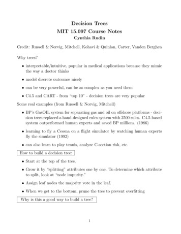
0.50.4EntropyGini index0.3Misclassification error0.20.10.00.00.20.40.60.81.0pNode impurity measures for two-class classification, as a function of theproportion p in class 2. Cross-entropy has been scaled to pass through(0.5, 0.5).Image by MIT OpenCourseWare, adapted from Hastie et al., The Elements of StatisticalLearning, Springer, 2009.C4.5 uses information gain for splitting, and CART uses the Gini index. (CARTonly has binary splits.)PruningLet’s start with C4.5’s pruning. C4.5 recursively makes choices as to whether toprune on an attribute: Option 1: leaving the tree as is Option 2: replace that part of the tree with a leaf corresponding to the mostfrequent label in the data S going to that part of the tree. Option 3: replace that part of the tree with one of its subtrees, correspondingto the most common branch in the splitDemoTo figure out which decision to make, C4.5 computes upper bounds on the probability of error for each option. I’ll show you how to do that shortly. Prob of error for Option 1 UpperBound1 Prob of error for Option 2 UpperBound210

Prob of error for Option 3 UpperBound3C4.5 chooses the option that has the lowest of these three upper bounds. Thisensures that (w.h.p.) the error rate is fairly low.E.g., which has the smallest upper bound: 1 incorrect out of 3 5 incorrect out of 17, or 9 incorrect out of 32?For each option, we count the number correct and the number incorrect. Weneed upper confidence intervals on the proportion that are incorrect. To calculate the upper bounds, calculate confidence intervals on proportions.The abstract problem is: say you flip a coin N times, with M heads. (Here Nis the number of examples in the leaf, M is the number incorrectly classified.)What is an upper bound for the probability p of heads for the coin?Think visually about the binomial distribution, where we have N coin flips, andhow it changes as p changes:p 0.5p 0.1p 0.9We want the upper bound to be as large as possible (largest possible p, it’s anupper bound), but still there needs to be a probability α to get as few errors aswe got. In other words, we want:PM Bin(N,preasonable upper bound ) (M or fewer errors) α11