WIXLIB

Risk aversionExpected utilityMeasuring risk aversionAbsurd implicationsInsurance choicesReference dependenceReferencesWhat is going on? Johnny’s choice implies:0.5u(w 11) 0.5u(w 10) u(w )) u(w 11) u(w ) u(w ) u(w 10) On average, Johnny values each dollar between w and w 11 by at most1011asmuch as the dollars between w 10 and w . Diminishing marginal utility (concavity) implies that the marginal dollar at w 10is at least as valuable as the marginal dollar at w . Similarly, the marginal dollar at w is at least as valuable as the marginal dollar atw 11 Taken together, this implies that Johnny values the dollar w 11 by at most1011as much as he values the dollar w 10.25

Risk aversionExpected utilityMeasuring risk aversionAbsurd implicationsInsurance choicesReference dependenceReferencesWhat is going on? (cont’d) Johnny makes the same choice when he is 21 richer:0.5u(w 21 11) 0.5u(w 21 10) u(w 21)) u(w 32) u(w 21) u(w 21) u(w 11) On average, he values each dollar between w 21 and w 32 by at most1011asmuch as the dollars between w 11 and w 21. Concavity implies that Johnny value the dollar w 32 by at most1011as much ashe values the dollar w 11.2 Hence he values the dollar w 32 by at most ( 1011 ) ˇ56as much as he values thedollar w 10.26

Risk aversionExpected utilityMeasuring risk aversionAbsurd implicationsInsurance choicesReference dependenceReferencesIterating this forward gives absurd implications! Rejecting the 50-50 lose 10/gain 11 gamble implies a 10 percent decline inmarginal utility for each 21 in additional lifetime wealth. 42 richer: (10/11)2 ˇ 5/6 420 richer: (10/11)20 ˇ 3/20 840 richer: (10/11)80 ˇ 2/100. Marginal utility plummets for substantial changes in lifetime wealth. You care less than 2% as about an additional dollar when you are 900 wealthierthan you are now.27

Risk aversionExpected utilityMeasuring risk aversionAbsurd implicationsInsurance choicesReference dependenceReferencesAbsurd implications! American Economic Association. All rights reserved. This content is excluded from our Creative Commons license. For moreinformation, see https://ocw.mit.edu/help/faq-fair-use/28

Risk aversionExpected utilityMeasuring risk aversionAbsurd implicationsInsurance choicesReference dependenceReferencesMeasuring risk aversion: preliminary summary Expected utility is the workhorse model for studying economic behavior under risk. Many important phenomena can be explained using this model. Example 1: investment behavior (fnance) Example 2: criminal behavior and risk of getting caught Coeÿcient of (relative) risk aversionis a key parameter of this model. Depending on the size of the gamble, we get very di erent answers for ! Small-scale gambles: people are very risk-averse. Large-scale risk: people are moderately risk-averse. The expected utility model can’t match both behaviors with only one parameter Rabin (2000) formalizes this issue. Recitation will discuss it a bit more.29

Risk aversionExpected utilityMeasuring risk aversionAbsurd implicationsInsurance choicesReference dependenceReferencesHow can we estimate ? Suppose you have a CRRA utility function:x 1 1 for6 1,ln xfor 1(u(x ) Three approaches to estimate :(1) Certainty equivalents(2) Choices from gambles(3) Insurance choices30

Risk aversionExpected utilityEstimatingMeasuring risk aversionAbsurd implicationsInsurance choicesReference dependenceReferencesusing insurance choices (Sydnor, 2010) Some doubts about validity of choices in lab games Would like to have real-world choices Sydnor (2010): data from large home insurance provider Random sample of 50,000 standard policies Policy parameters and claims fled over a one-year period Old and new customers What is a deductible? Expenses paid out of pocket before insurer pays any expenses Used to deter large number of claims31

American Economic Association. All rights reserved. This content is excluded from ourCreative Commons license. For more information, see https://ocw.mit.edu/help/faq-fair-use/Sample dataPolicyholder 1: Home was built in 1966 and had an insured value of 181,700.The menu available to this policyholder in the sample year was:Deductible 1,000 500 250 100Premium 504 588 661 773Relative to 1,000 policy0 84 157 269ChosenxPolicyholder 2: Home was built in 1992 and had an insured value of 266,100.The menu available to this policyholder in the sample year was:Deductible 1,000 500 250 100Premium 757 885 999 1,171Relative to 1,000 policy0 128 242 414ChosenxPolicyholder 2 had a higher premium for the 1,000 deductible contract thanPolicyholder 1, largely because Policyholder 2 had a higher insured home value.Policyholder 2, then, also faced a greater increase in cost for the alternative of a Choice over a menu of fourdeductibles 1, 000 500 250 100 Observe individuals’ choice setsand their preferred option32

Risk aversionExpected utilityMeasuring risk aversionAbsurd implicationsInsurance choicesReference dependenceReferencesChoosing a deductible What do these choices tell us about risk aversion? Losses to the customer are capped at the deductible. Choosing a lower deductible represents modest increase in insurance. Choice of low deductible thus reveals high risk aversion. What info do we need to learn about risk aversion? Available deductiblesPremium for each optionClaim probabilitiesWealth levels33

Risk aversionExpected utilityMeasuring risk aversionAbsurd implicationsInsurance choicesReference dependenceReferencesClaim rates are low: about 4 percent per yearTable 1—Summary StatisticsChosen deductibleVariableFullsample 1,000 500 250 ,679.50(4,584.58)709.78(269.34)1490.30Panel A. Selected policy variablesInsured home valueYear home was builtNumber of years insuredby the companyAverage age of household(H.H.) membersNumber of paid claims insample year (claim rate)Company payout per claimabove deductible levelYearly premium paidObservationsPercent of sampleNotes: Means with standard deviations are in parentheses. The average age measure was calculated by the insurancecompany based on information they have about household members. This variable is not used in rating. Insuredhome value is the coverage limit on the insurance policy. For the claim rate and payout by the company per claim,only claims that resulted in positive payouts by the company were counted. American Economic Association. All rights reserved. This content is excluded from our Creative Commons license. For more information, seehttps://ocw.mit.edu/help/faq-fair-use/34

Risk aversionExpected utilityMeasuring risk aversionAbsurd implicationsInsurance choicesReducing the deductible is expensive.Chosen deductibleAvailabledeductibleFullsample 1,000 500 250 100 615.82(292.59) 99.91(45.82) 86.59(39.71) 133.22(61.09) 798.63(405.78) 130.89(64.85) 113.44(56.20) 174.53(86.47) 615.78(262.78) 99.85(40.65) 86.54(35.23) 133.14(54.20) 528.26(214.40) 85.14(31.71) 73.79(27.48) 113.52(42.28) 467.38(191.51) 75.75(25.80) 65.65(22.36) 101.00(82.57)Reference dependenceReferences The average insurance pricewith a deductible of 1, 000is 615.82.Panel B. Deductible-premium menu 1,000 500 250 100 On average, reducing thedeductible from 1, 000 to 500 costs 99.91. On average, reducing thedeductible from 250 to 100 costs 133.22! American Economic Association. All rights reserved. This content is excluded from our Creative Commons license. For moreinformation, see https://ocw.mit.edu/help/faq-fair-use/35

Risk aversionExpected utilityMeasuring risk aversionAbsurd implicationsInsurance choicesReference dependenceReferencesPercent of customers holding each deductible levelYet the majority chooses small deductibles.90 1,00080 500 25070 10060504030201000–33–77–1111–1515 Number of years insured with companyFigure 1. Deductible Choice by Years Insured with Companynotes: This chart gives the fraction of customers holding each deductible level by groups of tenure with the company. The percent of the sample that falls into each category is as follows: 0–3 years (34.16 percent), 3–7 years(22.97 percent), 7–11 years (12.95 percent), 11–15 years (10.48 percent), 15 years (19.44 percent). American Economic Association. All rights reserved. This content is excluded from our Creative Commons license. For moreinformation, see https://ocw.mit.edu/help/faq-fair-use/36

Risk aversionExpected utilityMeasuring risk aversionAbsurd implicationsInsurance choicesReference dependenceReferencesChoosing a deductible Choice between one-year insurance contracts with yearly premium P anddeductible D Assumptions No other risk to lifetime wealth At most one loss during the year, with probability ˇ Accurate subjective beliefs about the likelihood of a loss Individuals maximize expected (indirect) utility-of-wealth function:V (w , P, D, ˇ) ˇ {z}prob(loss)· u(w P D) (1 ˇ) · u(w P) {zutility(loss)} {z } {z(1)}prob(no loss) utility(no loss)37

Risk aversionExpected utilityMeasuring risk aversionAbsurd implicationsInsurance choicesReference dependenceReferencesBacking out implied risk aversion from choices Choose contract j that maximizes expected (indirect) utility:max ˇ · u(w Pj Dj ) (1 ˇ) · u(w Pj ).j(2) Choices imply upper and lower bounds on risk aversion Upper bound for those who choose the 1,000 deductible Upper & lower bound for those who choose 500 or 250 deductible Lower bound for those who choose 100 deductible38

Risk aversionExpected utilityMeasuring risk aversionAbsurd implicationsInsurance choicesReference dependenceReferencesExample: Individual chooses 100 deductible The person prefers a 100 deductible over choosing a 250 deductible:V (w , P100 , 100, ˇ) ˇ ·(w P100 100)1 (w P100 )1 (1 ˇ) ·1 1 V (w , P250 , 250, ˇ) ˇ ·(w P250 250)1 (w P250 )1 (1 ˇ) ·1 1 Solving this equation yields lower bound for(for given P100 , P250 , w , and ˇ). Choosing a 100 deductible maximizes the available insurance. This choice reveals very high risk aversion in the expected utility framework. There are no options with even lower deductibles available, so we don’t know whatshe would have chosen for such deductibles.for this person. We thus don’t have an upper bound for39

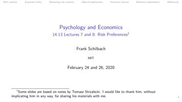
Risk aversionExpected utilityImplied values of190Measuring risk aversionAbsurd implicationsInsurance choicesReference dependenceReferencesare enormous!American Economic Journal: applied economics october 2010Table 3—Bounds on Coefficient of Relative Risk AversionModel 1,000(n 2,474)LB    UB 500(n 3,424)LB    UB 250(n 367)LB    UBReject any50/50 gamblewith potentialloss of 1,000Panel A. Bounds at the fiftieth percentile1 CRRA; 1 mil;deductible average2 CRRA; 1mil;individual estimate3 CRRA; 500k;individual estimate4 CRRA; IHV;individual estimate5 CRRA; 100k;individual estimate6 CRRA; 50k;individual estimate7 CRRA; 5k;individual estimate8 CARA; 1mil;individual estimateMode wealth 9832,0155,4114,62614,66199.9% 1,000(n 2,474)LB    UB 500(n 3,424)LB    UB 250(n 367)LB    UBReject any50/50 gamblewith potentialloss of 1,000Panel B. Bounds at the twenty-fifth and seventy-fifth percentile1 CRRA; 1 mil;deductible average—3,1731,6145,5823,89815,283100.0% Table shows lower and upperbounds at the 50th percentile. Di erent rows show estimatesfor di erent assumption onutility function and wealth. Example: for w 50k andCRRA utility, almost allestimates yield 100! American Economic Association. All rights reserved.This content is excluded from our Creative Commonslicense. For more information, seehttps://ocw.mit.edu/help/faq-fair-use/40

Risk aversionExpected utilityMeasuring risk aversionAbsurd implicationsInsurance choicesReference dependenceReferencesWhy do people choose small deductibles? Neoclassical explanations Sydnor (2010) discusses several potential explanations in Section IV of the paper. High risk aversion: implies implausibly high values of (see above). High objective probability of claims: but actual claim rates are low (around 4%). Borrowing constraints: unlikely given that people have fairly expensive homes. None of these explanations plausibly explains the patterns in the data.41

Risk aversionExpected utilityMeasuring risk aversionAbsurd implicationsInsurance choicesReference dependenceReferencesWhy do people choose small deductibles? Behavioral explanations Sydnor (2010) also argues that several behavioral explanations are unlikely. Risk misperception: requires people to vastly overestimate risk, including many whohave been insured for over 15 years with this company. Marketing, social pressure: possible but company is not a low-cost provider, so salesagents often suggest high deductibles to lower policy costs. Menu e ects (people avoid extreme options): possible but does not explain whypeople choose 250 rather than 500 deductibles. Preferred explanation: reference-dependent preferences/loss aversion (next)42

Risk aversionExpected utilityMeasuring risk aversionAbsurd implicationsInsurance choicesReference dependenceReferencesSummary from risk preferences Choices involving small-scale and large-scale risks yield contradicting answers.(1) Individuals are risk-averse for small-scale risks. Such choices imply enormous risk aversion for large-scale risks. But individuals do not avoid large-scale risks at all costs.(2) Individuals are moderately risk-averse for large-scale risks. Such choices imply that individuals should be nearly risk-neutral for small-scale risks. But individuals exhibit risk aversion for small-scale risks! Kahneman and Tversky (1979) Even more evidence against the expected utility model Proposed alternative model, reference-dependent utility (loss aversion), canexplain individuals’ risk attitudes for both small-scale and large-scale risks.43

(iii) RiskMeasuringAversion:u is concave(u" 0). Insurance choicesrisk aversionAbsurd implicationsReference dependenceReferencesA person is risk averse if he prefers the certain prospect (x) to any risky prospectwith expectedx. In expected utility theory, risk aversion is equivalent to theKahneman andTverskyvalue(1979)concavity of the utility function. The prevalence of risk aversion is perhaps thebest known generalization regarding risky choices. It led the early decisiontheorists of the eighteenth century to propose that utility is a concave function of Surveymoney,responsesstudentsand universityfacultyand bythisIsraeliin modernidea hasbeen retainedtreatments (Pratt [33], Arrow[4]). ‘Essentially identical’ results in Stockholm and MichiganIn the following sections we demonstrate several phenomena which violatethese tenets of expected utility theory. The demonstrations are based on the Series of hypothetical, large-stake choices such as this one:responses of students and university faculty to hypothetical choice problems. Therespondents were presented with problems of the type illustrated below.Which of the following would you prefer?Risk aversionExpected utilityA:50% chance to win 1,000,B: 450 for sure.50% chance to win nothing;The outcomes refer to Israeli currency. To appreciate the significance of theamounts involved, note that the median net monthly income for a family is about3,000 Israeli pounds. The respondents were asked to imagine that they wereactually faced with the choice described in the problem, and to indicate the44

268Risk aversionExpected utilityAND A. TVERSKYD. KAHNEMANMeasuring risk aversionAbsurd implicationsInsurance choicesReference dependenceReferencesThe Reflection EffectGains and lossesThe previous section discussed preferences betweenpositive prospects, i.e.,prospects that involve no losses. What happens when the signs of the outcomes are heircolumn ofTableIThe fnalleft-handlosses?are replacedreversedso thatgains peopledisplaysfour of the choice problems that were discussed in the previous section,associatedprobabilities).and the right-hand column displays choice problems in which the signs of the KahnemanandareTverskystrikingevidencethis predictionWe use -xto denotereversed.(1979):the loss contradictingof x, and to denotetheoutcomesprevalent preference, i.e., the choice made by the majority of subjects.TABLE IPREFERENCES BETWEEN POSITIVE AND NEGATIVE PROSPECTSPositive prospectsProblem 3:N 95Problem 4:N 95Problem 7:N 66Problem 8:N 66Negative prospects(4,000, .80) (3,000).[20][80]*(4,000, .20) (3,000, .25).[35][65]*(3,000, .90) (6,000, .45).[86]*[14](3,000, .002) (6,000, .001).[27][73]*Problem 3':N 95Problem 4':N 95Problem 7':N 66Problem 8':N 66(-3,000).(-4,000, .80) [8][92]*(-4,000, .20) (-3,000, .25).[58][42](-3,000, .90) (-6,000, .45).[8][92]*(-3,000, .002) (-6,000, .001).[70]*[30]In each of the four problems in Table I the preference between negative The EconometricSociety. Allrightsreserved.Thisis excludedbetweenfrom ourpositiveCreative prospects.Commons license.ofcontentThus, For morethe preferenceprospectsis themirrorimageinformation, see https://ocw.mit.edu/help/faq-fair-use/th

Psychology and Economics . 14.13 Lectures 7 and 8: Risk Preferences. 1. Frank Schilbach . MIT. February 24 and 26, 2020 . 1. Some slides are based on notes by Tomasz Strzalecki. I would like to thank him, without implicating him in any way, for sharing his materials with me. 1