Transcription
Introduction to Geostatistics — Course NotesYe ZhangDept. of Geology & GeophysicsUniversity of WyomingDraft date January 12, 2011
ContentsContents0.1 Overview . . . . . . . . . . . . . . . . . . . . . . . . . . . . . . .iiv1 Overview1.1 Why Geostatistics? . . . . . . . . . . . .1.2 Geostatistical Prediction . . . . . . . . .1.3 Geostatistics versus Simple Interpolation1.4 Limitations . . . . . . . . . . . . . . . .1.5 This Class . . . . . . . . . . . . . . . . .1.5.1 References . . . . . . . . . . . . .1.5.2 Outline . . . . . . . . . . . . . .1.5.3 Homework, Grades, Tools . . . .1.6 Suggested Reading . . . . . . . . . . . .1124699121212.15151616182020202223242425252628312 Probability Theory Review2.1 Nomenclature and Notation . . . . . . .2.2 Univariate Analysis . . . . . . . . . . . .2.2.1 Introduction . . . . . . . . . . .2.2.2 Formal Definitions . . . . . . . .2.2.3 Random Variable Arithmetic . .2.3 Bivariate Analysis . . . . . . . . . . . .2.3.1 Introduction . . . . . . . . . . .2.3.2 Bivariate Random Variables . . .2.3.3 Bivariate Arithmetics . . . . . .2.4 Multivariate Analysis . . . . . . . . . . .2.4.1 Linear Combination of Many r.v.2.4.2 Multivariate Arithmetics . . . . .2.5 Gaussian Distribution . . . . . . . . . .2.6 Central Limit Theorem . . . . . . . . .2.7 Chapter Project . . . . . . . . . . . . .2.8 Suggested Reading . . . . . . . . . . . .i.
iiCONTENTS3 Spatial Analysis3.1 Conventional Analysis (Nongeostatistical) . . . . .3.1.1 Data Posting . . . . . . . . . . . . . . . . .3.1.2 Contour Map . . . . . . . . . . . . . . . . .3.1.3 Symbol Map . . . . . . . . . . . . . . . . .3.1.4 Indicator Map . . . . . . . . . . . . . . . .3.1.5 Moving Window . . . . . . . . . . . . . . .3.2 Spatial Continuity Analysis (Geostatistical) . . . .3.2.1 Experimental Variogram . . . . . . . . . . .3.2.2 h-Scatterplot . . . . . . . . . . . . . . . . .3.2.3 Variogram versus Univariate Statistics . . .3.2.4 Higher Dimensions & Statistical Anisotropy3.2.5 Pure Nugget Variogram . . . . . . . . . . .3.2.6 Standard Deviation of γ̂(h) . . . . . . . . .3.2.7 Irregular Data: Variogram Search Envelope3.2.8 Exploring Anisotropy . . . . . . . . . . . .3.2.9 Spatial Continuity Analysis: Outline . . . .3.2.10 Issues. . . . . . . . . . . . . . . . . . . . .3.3 Chapter Project . . . . . . . . . . . . . . . . . . .3.4 Suggested Reading . . . . . . . . . . . . . . . . . .33333334343435373942444651565760656772744 Variogram Modeling4.1 Basic Permissible Models . . . . . . . . . . . . . . . . . .4.1.1 Positive Definiteness . . . . . . . . . . . . . . . . .4.1.2 Basic Variogram Functions . . . . . . . . . . . . .4.1.3 1D Variogram Model—Statistical Isotropy . . . . .4.1.4 Higher Dimensional Model—Statistical Anisotropy4.1.5 Nested Model . . . . . . . . . . . . . . . . . . . . .4.2 Model-Fitting “Rules of Thumb” . . . . . . . . . . . . . .4.3 Chapter Project . . . . . . . . . . . . . . . . . . . . . . .4.4 Suggested Reading . . . . . . . . . . . . . . . . . . . . . 1195 Estimation5.1 The Problem of Estimation . . . . . . . . . .5.2 Nongeostatistical (Deterministic) Estimation5.2.1 Global Estimation . . . . . . . . . . .5.2.2 Local Estimation . . . . . . . . . . . .5.3 Estimation Criteria . . . . . . . . . . . . . . .5.4 Geostatistical (Probabilistic) Estimation . . .5.4.1 Random Function Models . . . . . . .5.4.2 Ordinary Kriging . . . . . . . . . . . .5.4.3 Cokriging & Collocated Cokriging . .5.4.4 Kriging with moving neighborhood . .5.5 Chapter Project . . . . . . . . . . . . . . . .5.6 Suggested Reading . . . . . . . . . . . . . . .
CONTENTS6 Advanced Topics6.1 Cross Validation . . . . . . . . . . . .6.2 Other Estimators . . . . . . . . . . . .6.2.1 Simple Kriging . . . . . . . . .6.2.2 Indicator Kriging . . . . . . . .6.2.3 Block Kriging . . . . . . . . . .6.3 Geostatistical Simulation . . . . . . .6.3.1 Cholesky Decomposition . . . .6.3.2 Conditional Simulation . . . .6.3.3 Sequential Gaussian Simulation6.4 Chapter Project . . . . . . . . . . . .6.5 Suggested Reading . . . . . . . . . . .iii.1211211221221241261271301331361391417 Final Project7.1 Overview . . . . . . . . . . . . . . . . . . . . . . . . . . . . . . .7.2 What to hand in . . . . . . . . . . . . . . . . . . . . . . . . . . .7.3 Additional notes . . . . . . . . . . . . . . . . . . . . . . . . . . .1431431461488 Geostatistics Final Exam149. . . . . . . . . . . . . . . . . . . . . . . . .(SGS). . . . . . .
ivCONTENTSThis is the lecture note written & assembled by Ye Zhang for an introductorycourse in Geostatistics.Fall 2010GEOL 54463 CREDITSA-F GRADINGPre-requisite: Calculus I & II; Linear Algebra; Probability & Statistics;Matlab programming languageLocation: ESB1006Times: TTh (9:35 am 10:50 pm)Office hour: M(4:00 5:30 pm), F(3:00 4:30 pm), GE 220Email: yzhang9@uwyo.eduPhone: 307-766-2981The syllabus: see handout.NOTE: The lecture note do not include: (1) solutions to the exercises and projects; (2) proofs to theories and equation derivations.These will be presented only during lectures. So, please do not relyon the notes for everything — class attendance and participation arekey to doing well.0.1OverviewGeoscientists often face interpolation and estimation problems when analyzingsparse data from field observations. Geostatistics is an invaluable tool that canbe used to characterize spatial or temporal phenomena1 . Geostatistics originated from the mining and petroleum industries, starting with the work byDanie Krige in the 1950’s and was further developed by Georges Matheron inthe 1960’s. In both industries, geostatistics is successfully applied to solve caseswhere decisions concerning expensive operations are based on interpretationsfrom sparse data located in space. Geostatistics has since been extended tomany other fields in or related to the earth sciences, e.g., hydrogeology, hydrology, meteorology, oceanography, geochemistry, geography, soil sciences, forestry,landscape ecology. In this class, both fundamental development of geostatisticsand simple, practical applications in the earth sciences will be presented. Exercises and projects are designed to help elucidate the fundamental concepts.Reading assignments will be given illustrating the applications of geostatisticsin the particular field of reservoir characterization and modeling.1 In this class, we’re concerned only with spatial analysis; temporal phenomena might bebetter understood in a separate class on time series analysis.
Chapter 1OverviewWhat is geostatistics? Data analysis and spatial continuity modeling (Journel,1989). Establish quantitative measure of spatial correlation to be used for subsequent estimation and simulation (Deutsch, 2002). The following introductionand overview materials are based on compilation of several source materials (seefull references in Sec. 1.5.1).1.1Why Geostatistics?Classic statistics is generally devoted to the analysis and interpretation of uncertainties caused by limited sampling of a property under study. Geostatisticshowever deviates from classic statistics in that Geostatistics is not tied to apopulation distribution model that assumes, for example, all samples of a population are normally distributed and independent from one another. Most ofthe earth science data (e.g., rock properties, contaminant concentrations) oftendo not satisfy these assumptions as they can be highly skewed and/or possessspatial correlation (i.e., data values from locations that are closer together tendto be more similar than data values from locations that are further apart).To most geologists, the fact that closely spaced samples tend to be similar isnot surprising since such samples have been influenced by similar physical andchemical depositional/transport processes.Compared to the classic statistics which examine the statistical distributionof a set of sampled data, geostatistics incorporates both the statistical distribution of the sample data and the spatial correlation among the sample data.Because of this difference, many earth science problems are more effectively addressed using geostatistical methods. As stated by Marc Cromer (in Geostatistics for environmental and geotechnical applications, 1996, ASTM International,edited by Rouhani et al.):Geostatistical methods provide the tools to capture, through rigorous examination, the descriptive information on a phenomenon from sparse, often biased,and often expensive sample data. The continued examination and quantitative1
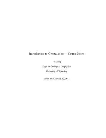
2CHAPTER 1. OVERVIEWrigor of the procedure provide a vehicle for integrating qualitative and quantitative understanding by allowing the data to “speak for themselves”. In effect, theprocess produces the most plausible interpretation by continued examination ofthe data in response to conflicting interpretations. . The application of geostatistics to environmental problems (e.g., groundwater contaminant cleanup)has also proven a powerful integration tool, allowing coordination of activitiesfrom field data acquisition to design analysis. For example, data collection isoften incomplete, resulting in uncertainties in understanding the problem andincreasing the risk of regulatory failure. While this uncertainties can often bereduced with additional sampling, the benefits must be balanced with increasingcost. . Thus, geostatistics offers a means to quantify uncertainty,while leveraging existing data to support sampling optimization.1.2Geostatistical PredictionThe goal of geostatistics is to predict the possible spatial distribution of a property. Such prediction often takes the form of a map or a series of maps. Twobasic forms of prediction exist: estimation (Figure 1.1) and simulation (Figure 1.2). In estimation, a single, statistically “best” estimate (map) of thespatial occurrence is produced. The estimation is based on both the sampledata and on a model (variogram) determined as most accurately representingthe spatial correlation of the sample data. This single estimate or map is usually produced by the kriging technique. On the other hand, in simulation, manyequal-likely maps (sometimes called “images”) of the property distribution areproduced, using the same model of spatial correlation as required for kriging.Differences between the alternative maps provide a measure of quantifying theuncertainty, an option not available with kriging estimation.Geostatistics has played an increasing role in both groundwater hydrologyand petroleum reservoir characterization and modeling, driven mainly by therecognition that heterogeneity in petrophysical properties (i.e., permeability andporosity) dominates groundwater flow, solute transport, and multiphase migration in the subsurface. Geostatistics, by transforming a sparse data set fromthe field into a spatial map (kriging estimation), offers a means to recreate heterogeneity to be incorporated into numerical flow and transport modeling. Onthe other hand, by transforming a sparse data set into multiple spatial maps(unconditional/conditional simulations), it offers a means of evaluating the uncertainties on modeling due to the uncertain nature of each map (Figure 1.3). Inboth reservoir simulation and groundwater modeling, for example, Monte Carlosimulation is a popular technique. Note that this uncertainty reflects our lackof knowledge about the subsurface, though the geological “groundtruth”, albeitunknown, is deterministic and certain.
1.2. GEOSTATISTICAL PREDICTION3Geostatistical EstimationExperimental VariogramSample Data Setγ (h)hKriging is an exactinterpolator (at sampledlocations, known datavalues are exactlypreserved)reality (unknown)!1010Variogram Modeling2020γ re 1.1: Geostatistical estimation workflow.Geostatistical SimulationSample Data Setγ (h)Variogram ModelingHistogramhreality (unknown)!Realization 1Realization 2Realization nFigure 1.2: Geostatistical simulation workflow.
4CHAPTER 1. OVERVIEWFlow Predictions Using Realizationsof a Geostatistical SimulationwateroilRealization 1wateroilwateroilRealization 2Realization nMeanPerformance Evaluation& Uncertainty AnalysisCumulativeOil ProducedTimeFigure 1.3: Flow predictions based on the realizations generated in a geostatistical simulation, e.g., Figure 1.2.1.3Geostatistics versus Simple InterpolationIn geostatistical estimation, we wish to estimate a property at an unsampledlocation, based on the spatial correlation characteristics of this property andits values at existing sampled locations. But, why not just use simple interpolation? How is spatial correlation incorporated in the geostatistical approach?A simple example may illustrate this point more clearly (Figure 1.4): we knowpermeability at n sampled locations, we wish to estimate the permeability atan unsampled location, z0 . Using inverse distance, the unknown value can beevaluated as:z0 nXwi zi(estimate)i 11/dii 1 (1/di )wi Pn(weight)We can see that the above relation is a linear estimator, i.e., z0 is a weighted sumof the n known values. Each weight (wi ) (assigned to a known zi ) is determinedby the distance of the known data point to the unknown data point. For n 7,for example, the weights can be calculated easily as shown in Figure 1.5.Using this scheme, the weights assigned to points 1, 2, 4, 6 are all equal to0.2. However, from the understanding of geology, we realize that permeability
1.3. GEOSTATISTICS VERSUS SIMPLE INTERPOLATION5Z is permeability:z0: unknown value to be estimatedzi (i 1, ., n): a set of known measurementsyznz5xz4z0 ?SandClayz6z1z3z2Figure 1.4: Estimation of the unknown permeability z0 based on a set of knownvalues of permeability at n locations.z0: unknown value to be estimatedzi (i 1, ., 7): a set of known measurementsz7 (0.06)yxd5z4 (0.2)d4z1 (0.2)z5 (0.07)d7d1z0 ? d6d2z2 (0.2)z6 (0.2)d3z3(0.07)Figure 1.5: Estimation of the unknown z0 given 7 known values. Numbers inparenthesis are weights assigned to the known values based on inverse distance.
6CHAPTER 1. OVERVIEWwithin the elongated sand body should be more similar in the lateral direction.Thus, points 4 and 6 should be given higher weights than points 1 and 2. This isobviously not the case when using inverse distance. Thus, in conventional interpolation methods (e.g., inverse distance, inverse distance squared), informationon spatial correlation is not incorporated. On the other hand, geostatisticalestimation considers both distance and spatial correlation. In general, geostatistical estimation consists of 3 steps: (1) examining the similarity between aset of sample (known) data points via an experimental variogram analysis; (2)fitting a permissible mathematical function to the experimental variogram; (3)conducting kriging interpolation based on this function. In the above example,the spatial correlation will be revealed by the more similar values of z4 and z6(step (1)). It will be modeled via step (2) (variogram modeling). Then, usingkriging, we’ll find that the weights assigned to points 4 and 6 will increase (thoseof 1 and 2 will decrease accordingly since the total weight must sum to 1.0) (step(3)). In kriging, based on the new weights, a best linear unbiased estimate of z0is obtained. Further (though sometimes optional depending on the goal of thestudy), uncertainty in the estimated field is additionally evaluated. In this class,we’ll use many exercises to illustrate how to conduct a geostatistical study.Given the same set of sampled data, interpolation results using IDS (di isreplaced by d2i ) and kriging can look drastically different (Figure1.6). However,does this mean that kriging is the preferred interpolation method regardless ofthe data? It turns out, there are situations when the sampled data are simplynot good for kriging (we’ll explore this aspect when we look at the “pitfalls” ofconducting a variogram analysis). Given such data—either too unreliable or toosparse and widely spaced to capture the spatial correlation of the true propertyfield, the conventional IDS may give just as good result. The decision of whichmethod to use is in a way data-driven. Usually, an increase in sample qualityor density will affect which method may be the most appropriate for the study.1.4LimitationsWhat is not geostatistics?Interestingly, geostatistics models mathematical objects, not geological objects. For example, given a set of spatial measurements of isopach values, ageologist can create various contour maps based on his/her understanding ofthe underlying geology (Figure 1.7). This process is best described as patternrecognition—the geologist has an existing idea of the underlying geology whendoing the interpretation. Geostatistics, however, does not recognize pattern,rather, it is based on a set of mathematical principles.As stated by AndréJournel (1989), “geostatistics is an art, and as such,is neither completely automatable nor purely objective”. In an experimentconducted by the US EPA, 12 independent geostatisticians were given the samedataset and asked to perform the same kriging. The 12 results were very differentdue to widely different data analysis conclusions, variogram models, choices of
1.4. LIMITATIONS7Figure 1.6: Estimation results from IDS and Kriging, based on the same set ofsample data.
8CHAPTER 1. gure 1.7: A geologist’s interpretations of isopach data (after Chiles & Delfiner,1999): (a) meandering channel; (b) in-fill channel; (c) paleovalleys; (d) barrierbar and tidal channel.
1.5. THIS CLASS9kriging type, and search strategy. As stressed by Journel, “that there are noaccepted universal algorithm for determining a variogram/covariance model,that cross-validation is no guarantee that an estimation procedure will producegood estimates at unsampled locations, that kriging needs not be the mostappropriate estimation method, and that the most consequential decisions ofany geostatistical study are made early in the exploratory data analysis”.In this class, I will repeatedly emphasize the importance of understanding our data, via exploratory analysis, trend analysis, error identification, anddealing with sampling issues and non-stationarity. From both the environmental engineering and petroleum reservoir modeling literature, I present “rules ofthumb” or “best practice” guide that is recommended by experts in the field.Further, it is my recommendation that before you embark on a geostatisticalstudy, you should research the literature for analysis conducted on similar datain the past. You can often learn a lot from past studies and hopefully, youcan try to avoid pitfalls that others had stumbled upon before you. In the endof this class, I will present a lecture on literature search and point to furtherresources that you can use to solve your own problems.Thus, geostatistics is not a black box. Without understandingits fundamental assumptions and limitations, an untrained person ismore likely use it incorrectly. As summarized by Journel (1989): Geostatistics is a tool: it cannot produce good results from bad data. It cannot replacecommon sense, good judgment, or professional insight. Throughout the course,I’ll pay equal attention to its limitations as well as its useful applications. Inpractice, as more data become available, the geostatistical procedure often needto be repeated, the data re-analyzed or reinterpreted.Another point to make is that estimation or simulation based on variogramscannot very well capture curvilinear features, e.g., curved channels (Figure 1.8).To overcome such limitations, recent development includes multiple point statistics (where correlation is characterized among multiple data points and thenincorporated into simulations), pluralGaussian simulation (several correlatedpopulations can be superimposed), and hybrid or hierarchical approaches (e.g.,kriging is used to create property distribution within a higher-order geobodycreated via either deterministic or stochastic means, often object-based). Theseare currently areas of active research.1.5This Class1.5.1ReferencesIn this class, a fairly rigorous mathematical treatment is presented. This courseis thus designed at the upper undergrad and graduate level, appropriate for thelevel of rigor contained herein. Course lecture is the key, though most materialsare assembled based on several textbooks, tutorials, and lecture notes, each withits own emphasis: Engineering Geostatistics, Course Notes, Randal Barnes, 2000, Depart-
10CHAPTER 1. OVERVIEW123NVariogram EW1.2Variogram ure 1.8: Experimental variograms computed for 3 different types of geologicalheterogeneity (from Caers and Zhang, 2002), illustrating the limitations of usingvariograms to describe heterogeneity with non-linear features.
1.5. THIS CLASS11ment of Civil Engineering, U of Minnesota. An Introduction to Applied Geostatistics, Isaaks & Srivastava (I&S), 1989,Oxford University Press. Geostatistical Reservoir Modeling, Clayton Deutsch, 2002, Oxford University Press. Fundamentals of Geostatistics in Five Lessons, Andre Journel, 1989, ShortCourse in Geology, vol 8, Presented at the 28th International GeologicalCongress, Washington, D. C. Introduction to Geostatistics, Application in Hydrogeology, Peter Kitanidis, 1997, Cambridge University Press. GSLIB: Geostatistical Software Library and User’s Guide, Clayton Deutsch& Andre Journel, 2nd Edition, Oxford University Press, 1997.Bear in mind that the current course can only serve an introductory purpose:it cannot hope to cover every aspect of the subject as presented in the references, nor will we have time to explore many advanced topics, as they are beingcontinuously developed and refined in the literature. In particular, the topicsof this course are limited to stationary random space function (RSF) (stationarity here, roughly speaking, means that the mean, variance, and variogram donot change with position in the data field; if we have time, we’ll cover SimpleKriging which is not based on assuming stationary RSF). Although there aregeostatistical estimation methods developed for non-stationary RSF, the mostwidely used ones are based on stationary RSF. Wikipedia has a listing of themajor kriging techniques used in practice:http://en.wikipedia.org/wiki/KrigingTo further be exposed to the power of the geostatistical analysis, we mighthave a guest lecturer to give a talk about the reservoir simulation workflow.Finally, all lectures are rooted in a fairly rigorous mathematical framework.Hopefully, such an approach will better prepare you for the more advancedtopics or doing independent research. The exercises are designed to help youunderstand both the strength of the geostatistical methods and the variouspitfalls you may encounter when working with raw data and the suggested solutions. The suggested reading list at the end of each chapter presents eitherexample applications of geostatistics in different geoscience specialties or selecttopics specific to geostatistical reservoir simulation. They are not specific tothe topics of each chapter, however, i.e., most papers are assuming you’re already familiar with the fundamentals. Some of these papers come from thepapers compiled in: Geostatistics for environmental and geotechnical applications, Shahrokh Rouhani et al. (editors), 1996, ASTM publication. Some comefrom excerpts of the textbook Geostatistical Reservoir Modeling by Deutsch(2002). I will also post additional papers on a ftp site that you can access.
12CHAPTER 1. OVERVIEW1.5.2OutlineThe outline of this course is:1. Probability Theory Review2. Spatial Analysis3. Experimental Variogram4. Variogram Modeling5. Geostatistical Estimation (Kriging & Co-Kriging)6. Geostatistical Simulation (Unconditional & Conditional)7. Advanced Topics1.5.3Homework, Grades, ToolsIn addition to exercises and projects, reading assignments are given, which maybe expected to be discussed during the class meeting if we have time. Forsome paper assignments, students are expected to produce a short (15 minute) powerpoint presentation on what has been learned from these papers. Thosewho do not show up in class or fail to participate in the exercises may expectF. Tools for simple exercises include ruler, calculator, Excel, Matlab. For morecomplex projects, we’ll use software packages such as Surfer (kriging estimation)and Gslib (stochastic simulation).1.6Suggested ReadingBesides the above textbooks, other reading materials may come from:1. Geostatistics for environmental and geotechnical applications: a technology transferred, M. V. Cromer, in Rouhani et al. (1996).2. Describing spatial variability using geostatistical analysis, R. M. Srivastava, in Rouhani et al. (1996).However, it is my belief that depending on the type of research you do, doliterature search, and focus on papers that have similar aspects to your problems.This might help you not get lost in the sea of the ever expanding geostatisticalliterature!Some final thoughts: This is a-graduate level class on a challenging subject. Instead of learning how to use some software, the course emphasizes fundamental and quantitative understanding. So, be prepared to think hard. Workout the exercises and projects yourself. Theoretical rigor is emphasized becauseI believe that if you do research related to spatial analysis, fundamental aspectsare important. You simply cannot hope to understand many literature papers
1.6. SUGGESTED READING13or produce quality results if you’re not exposed to a systematic study of the fundamental principles lying behind software applications. However, if you’re onlyinterested in applied problems, you may feel that theories and accompanyingderivations and programming (you’re required to write a few Matlab codes) aretoo tedious and not of interest to you. For those with such a view, please consider taking an alternative class with a more applied emphases. In this course,a series of chapter projects are designed using Surfer which shows the typicalsteps involved in applications of kriging, though solving applied problems is notthe focus. Make sure you sign up the class for the right reason.
14CHAPTER 1. OVERVIEW
Chapter 2Probability Theory ReviewWe review some basic concepts and results of probability theory that are ofrelevance. It is meant to be a refresher of concepts covered in a separate statisticscourse. However, in case you have not taken such courses, the concepts andresults will be explained using simple examples.2.1Nomenclature and Notation1. Important nomenclature: P r[A]—the probability of event A occurring;P r[A]—the probability of event A not occurring;P r[A B]—the probability of event A and event B both occurring;P r[A B]—the probability of event A or event B occurring;P r[A B]—the probability of event A occurring given that event Bhas occurred.2. Axioms: 0 P r[A] 1; P r[Ω] 1, Ω is the union of all possible outcomes.3. Conditional Probability:P r[A B] P r[A B]P r[B]4. Independence:Events A and B are statistically independent if and only if:P r[A B] P r[A] · P r[B]In words, if events are independent, the probability of their join occurrenceis simply the product of their individual probabilities of occurrence.15
16CHAPTER 2. PROBABILITY THEORY REVIEWDiscrete DistributionPi Pr[X xi]0.501 ( head )2 ( tail )xFigure 2.1: Outcomes of experiments of tossing a coin: discrete r.v. and itsprobability distribution.2.22.2.1Univariate AnalysisIntroductionOne may define the probability of an event as between 0 and 1, representing thechance or relative frequency of occurrence of the event. The probabilities of allpossible (mutually exclusive) events of an experiment must sum to 1. In practice,the outcomes of experiments are assigned numerical values, e.g., when tossing acoin, 1 and 2 can be assigned to the outcome of “head” and “tail”, respectively(Figure 2.1). Such numerical values can be represented by a Random variable(r.v.). Two types of r.v. exist: discrete and continuous. Discrete examplesinclude the outcome of tossing a coin (head or tail), the grades of this course(A, B, C, D, F); continuous examples include the height of all men in the U.S.(ranging from, say, 4 ft to 7 ft), the grades of a class (e.g., 0.0 100.0 points). Inthis class, a r.v. is expressed with a upper-case letter, e.g., X. The numericalvalue of a particular outcome is designated as the lower-case equivalent “x”.The probability of a r.v. occurring at any possible value (discrete r.v.)or within a range of values (continuous r.v.) is described by its probabilitydistribution. For discrete r.v., its distribution is also discrete (Figure 2.1):(2.1)Pi P r[X xi ],i 1, . . . , n.
2.2. UNIVARIATE ANALYSIS17Table 2.1: Grade distribution of a class. An example of a discrete r.v.Grades Number of People X xiA26B125C204D73E32F11In this case, P1 P r[X 1] 0.5, P2 P r[X 2] 0.5, and P1 P2 1.In the discrete r.v., its distribution is just the frequency (or proportio
statistics to environmental problems (e.g., groundwater contaminant cleanup) has also proven a powerful integration tool, allowing coordination of activities from fleld data acquisition to design analysis. For example, data collection is often incomplete, re