Transcription
Basic Statistics Made EasyVictor R. Prybutok, Ph.D., CQE, CQA, CMQ/OE, PSTAT Regents Professor of Decision Sciences, UNTDean and Vice Provost, Toulouse Graduate School, UNT13 October 2017
Agenda StatisticsStatistical MeasuresDistributionsRepeatability and Reproducibility (R&R)Process CapabilityStatistical Process ControlOctober 12 - 13, 201726th Annual ASQ Audit Division Conference: The IntercontinentalAddison2
Statistics Statistics deals with the collection, analysis, presentation and useof data to solve problems, design and develop products andprocesses, and make decisions Descriptive Statistics – organize, summarize and present data in an informative way– Describe and control VariabilityInferential Statistics–Reasoning and Generalization of results from a sample to a population Examples What is the percentage of products not meeting specifications?What is the tolerance of this product?Is this a stable process, and if not, how can we stabilize it?What is the probability that a lot of products will be rejected?Should the entire lot of 100,000 items be rejected if 10 out of 100 inspected itemswere found defective?October 12 - 13, 201726th Annual ASQ Audit Division Conference: The IntercontinentalAddison3
Population vs. Sample Population collection of objects of interest Sample portion of the population of interest Sampling sample selection methodsPopulationSample Statistics key measurement calculationsusing sample data (observations): e.g. Zstatistic; expressed as numbers Parameters population parameters to drawnconclusions about; can be expressed as:Sampling Parameter (unknown)Random sampling most commonly usedStatisticHypotheses: e.g. the average length is 10 ft.Confidence intervals (CI): e.g. the averagelength is between 9.45 ft. and 10. 55 ft. Statistical significance (α) probability ofmaking a (Type I) prediction error (e.g. α 5%) Acceptable margin of error in prediction Confidence Level (CL) 1- αStatistical Inference (Prediction) Statistical significance / Confidence Level October 12 - 13, 2017E.g. I am 95% confident that the averagelength is 10 ft.E.g. I am 95% confident that the averagelength is between 9.45 ft. and 10. 55 ft.26th Annual ASQ Audit Division Conference: The IntercontinentalAddison4
Sampling The sample reflects the characteristics of the population from whichit is drawn, otherwise a sampling error occurs– Increase sample size to reduce sampling error Random sampling: each item in the population has an equalprobability of being selected; most commonly used Stratified sampling: population partitioned into groups, and a sampleis selected from each group Systematic sampling: every nth (e.g.4th, 5th) item is selected Cluster sampling: population partitioned into groups (clusters), and asample of clusters is selected– Either all elements in the chosen clusters are selected, or a random sample istaken from each cluster selected Judgment sampling: expert opinion is used to determine the sampleOctober 12 - 13, 201726th Annual ASQ Audit Division Conference: The IntercontinentalAddison5
Data Types Variables are measurements ofcharacteristics of interest Qualitative or Attribute Variablesare not numeric Quantitative Variables are: Discrete Variables can onlytake particular, distinct values– No other values in-between– Counting / enumerating Continuous Variables canassume any value over acontinuous range– Infinite values in-between– MeasuringOctober 12 - 13, 201726th Annual ASQ Audit Division Conference: The IntercontinentalAddison6
Probabilities Probability is the likelihood that an event outcome occurs– 𝑃 𝐴 𝐶𝑜𝑢𝑛𝑡 𝑜𝑓 𝑒𝑣𝑒𝑛𝑡 𝑜𝑢𝑡𝑐𝑜𝑚𝑒 𝐴 �� 𝑛𝑢𝑚𝑏𝑒𝑟 � P(A) is a number between 0 and 1 Conditional Probability is the probability of event A given that event B hasalready occurred– 𝑃 𝐴𝐵 𝑃(𝐴 𝑎𝑛𝑑 𝐵)𝑃(𝐵)Multiplication Rule:– 𝑃 𝐴 𝑎𝑛𝑑 𝐵 𝑃 𝐴 𝐵 𝑃 𝐵 𝑃 𝐵 𝐴 𝑃 𝐴– Independent Events: P(A and B) P(A) * P(B) Addition Rule:– P(A or B) P(A) P(B) – P(A and B)– Mutually Exclusive Events: P(A and B) 0 Example:– 𝑃(test indicates defective and product is not defective) P(test indicates defective product is not defective) * P(product is not defective)October 12 - 13, 201726th Annual ASQ Audit Division Conference: The IntercontinentalAddison7
Data VisualizationMultivariate TestsaEffect TablesCharts / GraphsScatter PlotsFrequency Histograms and PolygonsProbability DistributionsOthers–InterceptValuePillai's TraceHypothesis dfError 00.000.000Hotelling's Trace15.4261028.410b6.000400.000.000Roy's Largest Root15.4261028.410b6.000400.000.000Pillai's Trace.1142.63718.0001206.000.000Wilks' Lambda.8882.68418.0001131.856.000Hotelling's .000.000Wilks' Lambdaq7F.939Roy's Largest RootStem and leaf, box plots, decision treesOctober 12 - 13, 201726th Annual ASQ Audit Division Conference: The IntercontinentalAddison8
Agenda StatisticsStatistical MeasuresDistributionsRepeatability and Reproducibility (R&R) AnalysisProcess CapabilityStatistical Process ControlOctober 12 - 13, 201726th Annual ASQ Audit Division Conference: The IntercontinentalAddison9
Distributional Shape SymmetrySkewness––– Modality– Negatively Skewed: tail points to the lowerend of the x axisPositively Skewed: tail points to the upperend of the x axisCoefficient of Skewness : -1 CS 1; CS 0 no skewnessBimodal, trimodal distributions, etc.Kurtosis––More or less peaked: leptokurtic,platykurticCoefficient of Kurtosis: CK 3 morepeaked; CK 3 more flatOctober 12 - 13, 201726th Annual ASQ Audit Division Conference: The IntercontinentalAddison10
Measures of Central Tendency Mode: the most frequently occurringscoreMedian: midpoint of the distribution ofscores; divides the distribution intotwo equally large partsMean (𝑥,ҧ μ): the average of all scoresMidrange: the average of lowest (L)and highest (H) scoresOctober 12 - 13, 201726th Annual ASQ Audit Division Conference: The IntercontinentalAddison11
Measures of Variability Variability: degree of dispersion among scores– Homogeneous (low variability)– Heterogeneous (high variability) Range (R): difference between the highest (H) and lowest (L) scoresVariance (s2, σ2)Standard Deviation (s, σ)Coefficient of Variation: CV 𝑥𝑠ҧ 100October 12 - 13, 201726th Annual ASQ Audit Division Conference: The IntercontinentalAddison12
Measures of Position Percentiles: degree of dispersion among scores– Q1 the 25th percentile value– Q2 the 50th percentile value the median– Q3 the 75th percentile value Interquartile Range: distance between the low and the high score forthe middle half of the data– IQR Q3 - Q1 Standard Scores: z-score and t-score are the most common– Every sample observation x has a corresponding z-score 𝑥 𝑥ҧ𝑠– Indicates how many standard deviations (s) a particular raw score x lies above orbelow the sample mean 𝑥ҧOctober 12 - 13, 201726th Annual ASQ Audit Division Conference: The IntercontinentalAddison13
Agenda StatisticsStatistical MeasuresDistributionsRepeatability and Reproducibility (R&R) AnalysisProcess CapabilityStatistical Process ControlOctober 12 - 13, 201726th Annual ASQ Audit Division Conference: The IntercontinentalAddison14
Normal (Gaussian) Distribution X is Normally distributed with mean µ andstandard deviation σ X N(µ, σ2)– The N(0,1) distribution is called Standard NormalDistributionStandard Normal Distribution––––––––Z is a random variable taking values z (z-scores)Enable easy calculations (using tables, Excel, calculator, etc.)P(Z 0.92) 0.8212 (from tables)Excel: P(Z 0.92) NORM.S.DIST (0.92, TRUE) 0.8212P(- z ) 1P(Z 0.92) 1-P(Z 0.92) 1-0.8212 0.1788P(Z 0) 0.5 P(z 0)P(-0.64 Z 0.43) P(Z 0.43) – P(z -0.64) 0.6664 – (1- 0.7389) 0.4053October 12 - 13, 201726th Annual ASQ Audit Division Conference: The IntercontinentalAddison15
Empirical Rule 68.3% of the distribution lies within1*σ from the mean μ 95.4% of the distribution lies within2*σ from the mean μ 99.7% of the distribution lies within3*σ from the mean μOctober 12 - 13, 201726th Annual ASQ Audit Division Conference: The IntercontinentalAddison16
Standardization and the Central LimitTheorem (CLT) Standardization: converts any normal distribution value to a standard𝑋 μnormal distribution value using the transformation Z σ– If X N(µ, σ2) and Z (X µ) / σ then Z N(0, 1)– If X N(3500, 500 ) calculate P(X 3100) P(X 3100) P[(X µ) / σ (3100 µ) / σ ] P[Z (3100-3500) / 500] , where Z N(0,1) P(Z -0.8) 0.2119 Central Limit Theorem (CLT)– If simple random samples of size n are taken from any population having a meanμ and standard deviation σ, the probability distribution of the sample meanapproaches a normal distribution– As n - the distribution of the variable Z ത𝑋 μ(σ)𝑛approaches standard normal, Z N(0, 1)– Pillar of statistical inference: allows using the sample mean distribution and itsparticular properties to make inferences about the populationOctober 12 - 13, 201726th Annual ASQ Audit Division Conference: The IntercontinentalAddison17
CLT IllustrationTheoretical DistributionSample Size 1Sample Size 10October 12 - 13, 2017Sample Size 2Sample Size 2026th Annual ASQ Audit Division Conference: The IntercontinentalAddison18
Importance of CLT In certain conditions (e.g. large sample size), one can approximateany distribution with a Normal distribution although the distribution isnot Normally distributed– Through sampling, distributions that are prohibitively difficult to define areapproximated by the sampling distribution of the mean which is a standardnormal distribution– Results can be generalized from sample to the population Allows inference from sample to population With a large enough sample, most of the sample means will be closeto the population mean Can determine probability that a certain sample mean falls within acertain distance from the population meanOctober 12 - 13, 201726th Annual ASQ Audit Division Conference: The IntercontinentalAddison19
Normal Distribution Example 1 The average length of steel bars produced by a constructioncompany has historically been 75 inches, with a standard deviationof 0.25 inch. If a sample of 49 steel bars is taken, what is theprobability that the sample mean is at least 75.05 inches? Solution– μ 75 in.; σ 0.25 in.; n 49– P(𝑋ത 75.05) ?– CLT Z ത𝑋 μ(σ)𝑛 N(0, 1)– P(𝑋ത 75.05) P(ത𝑋 μ(σ)𝑛 75.05 μ(σ)𝑛) P(Z 75.05 750.25)49() P(Z 1.4) 1-P(Z 1.4) 1-NORM.S.DIST(1.4, true) 0.0808October 12 - 13, 201726th Annual ASQ Audit Division Conference: The IntercontinentalAddison20
Normal Distribution Example 2 A manufacturer of MRI scanners has data that indicates that thenumber of days between scanner malfunctions is normallydistributed, with a mean of 1020 days and a standard deviation of 20days. What is the number of days for which the probability ofscanner malfunction is 0.8. Solution– μ 1020 days; σ 20 days; P(X x ) 0.8𝑥 μ– Standardization of x values using z Z N(0,1) and P(Z z ) 0.8 zσ NORM.S.INV(0.8) 0.84 x z*σ μ 0.84*20 1020 1036.8October 12 - 13, 201726th Annual ASQ Audit Division Conference: The IntercontinentalAddison21
Normal Distribution Example 3 Assume that the noise in a digital transmission system is normallydistributed with a mean of 0 Volts and a standard deviation of 0.45Volts. A digital “1” is transmitted when voltage exceeds 0.9 Volts.What is the probability of false detection at the receiving end?Determine symmetric bounds around 0 that include 99% of all noisereadings. Solution– μ 0; σ 0.45– False detection detect a digital “1” when none was sent noise 0.9 Voltswill wrongly be interpreted as digital “1”𝑥 μ0.9 μ0.9– P(X 0.9) P( ) P(Z ) P(Z 2) 1-P(Z 2) 1σσ0.45NORM.S.DIST(2, true) 0.02275– X noise P(-x X x) 99% standardization P(-z Z z) 99% P(Z z) – P(Z -z) 0.99 1- P(Z z) – P(Z -z) 0.99 1-2*P(Z -z) 0.99 P(Z -z) (1-0.99)/2 0.005 -z NORM.S.INV(0.005) -2.58 x z*σ μ 2.58*0.45 0 1.161 P(-1.161 X 1.161) 99%October 12 - 13, 201726th Annual ASQ Audit Division Conference: The IntercontinentalAddison22
Determining Sample Size (σ unknown) A telecommunications company claims that 90% of their voice & dataswitches still function after major data center floods when they were underwater for up to 8 hours. How many flooded switches have to be tested todetermine the true proportion with a 95% confidence interval 6% wide (i.e.margin of error 3%)? What should the sample size be if we decrease themargin of error from 3% to 2%? Solution:–CL 95% α 1-95% 0.05–Margin of Error: E 6%/2 0.03 𝑍α––Zα/2 NORM.S.INV(1-α/2) 1.96 (or from Z tables)𝑝Ƹ 90% from eq. (a) 𝑛 1 (𝑍α/2/E)2[𝑝(Ƹ 𝑝Ƹ 1)] 1 (1.96/0.03) 2*(0.9*0.1) 385.16 386 switches to be tested𝑛′ 1 (𝑍α/2/E’)2[𝑝(Ƹ 𝑝Ƹ 1)] 1 (1.96/0.02) 2*(0.9*0.1) 865.36 866 switches to betestedPrecision increases 1% (from 3% to 2%) larger sample size is needed (from 386 to 866)––2October 12 - 13, 2017Ƹ𝑝(1 𝑝)Ƹ𝑛 1(a)26th Annual ASQ Audit Division Conference: The IntercontinentalAddison23
Determining Sample Size (σ unknown) A semiconductor company manufactures military specification resistors. Wewant to know the average resistance of these special resistors, with amargin of error of 10%, and be 99% confident about our result. How manyspecial resistors should be inspected and measured? From previousstudies, we know σ is 3. What should the sample size be if we relax theconfidence level to 95%? Solution:–CL 99% α 1-99% 0.01–Margin of Error: E 10% 0.1 𝑘( ) (a)––––k Zα/2 NORM.S.INV(1-α/2) 2.576 (or from Z tables)From eq. (a) 𝑛 [k*(σ /E)]2 (2.576*3/0.1) 2 5972.2 5973 resistors to be measuredHigh confidence (99%) large sample size (5973)CL’ 99% α’ 1-95% 0.05 k’ Zα/2 NORM.S.INV(1-α’/2) 1.96 (or from Z tables) 𝑛′ [k’*(σ /E)]2 (1.96*3/0.1) 2 3457.44 3458 resistors to be measuredLower confidence (95%) smaller sample size needed (3458)––σ𝑛October 12 - 13, 201726th Annual ASQ Audit Division Conference: The IntercontinentalAddison24
Binomial Distribution Discrete probability of obtaining exactly x “successes” in a sequence of ntrials𝑛 𝑥𝑛!𝑝 𝑥 𝑝 1 𝑝 𝑛 𝑥 , 𝑥 0, 1, 2, . . 𝑛 𝑥! 𝑛 𝑥 ! 𝑝 𝑥 (1 𝑝)𝑛 𝑥 , 𝑥 𝑥0, 1, 2, 𝑛μ 𝑛𝑝, σ2 𝑛𝑝(1 𝑝)“Success” any one of two possible outcomes– E.g. Defective / non-defective , male / female, etc.p probability of “success”Excel: BINOM.DIST (x, n, p, TRUE)TRUE result is cumulative probabilityOctober 12 - 13, 201726th Annual ASQ Audit Division Conference: The IntercontinentalAddison25
Binomial Distribution Example The probability that a process produces a non-defective part is 0.8.What is the probability that 4 parts among a sample of 20 will bedefective? What is the probability that at least 1 part will bedefective? What is the expected (average) number of defective partsif the sample size is increased to 50? Solution:– “Success” defective part; p P(“success”) P(defective) 1-P(non-defective) 1-0.8 0.220!– x 4, n 20 P(4) 0.24 0.816 (17*18*19*20/24)*0.002*0.028 4! 16!0.218– EXCEL: P(4) BINOM.DIST(4, 20, 0.2, false) 0.218– P(X 1) 1-P(X 1) 1-P(0) 1- BINOM.DIST(0, 20, 0.2, false) 1-0.012 0.988– E(defective) μ n*p 50*0.2 10October 12 - 13, 201726th Annual ASQ Audit Division Conference: The IntercontinentalAddison26
Poisson Distribution Discrete probability of exactly x events occurring in a fixed interval (can betime, space, area, volume, etc.) if these events occur with a known averagerate λ (per interval) and independently of the time since the last event𝑝 𝑥 𝑒 λ λ𝑥𝑥! μ λ, σ2 λ λ average rate or expected number ofoccurrences Excel: POISSON.DIST (x, λ, TRUE) TRUE result is cumulative probabilityOctober 12 - 13, 201726th Annual ASQ Audit Division Conference: The IntercontinentalAddison27
Poisson Distribution: Example 1 The average number of non-conforming products found duringinspection is 12. What is the probability that exactly 5 nonconforming products are found? What is the probability that amaximum of 3 non-conforming units are found? What is theprobability that between 2 and 6 non-conforming units are found? Solution:– λ 12, x 5 P(5) POISSON.DIST(5, 12, false) 0.0127– P(X 4) POISSON.DIST(4, 12, true) 0.0076– P(2 X 6) P(X 6) – P(x 2) POISSON.DIST(6, 12, true) - POISSON.DIST(2,12, true) 0.045822-0.000522 0.0453October 12 - 13, 201726th Annual ASQ Audit Division Conference: The IntercontinentalAddison28
Poisson Distribution: Example 2 5 sheets of polished metal are examined for scratches and theresults are given in the table below. What is the probability offinding no scratches per square inch? What is the probability ofchoosing a sheet at random that contains 4 or more scratches? Solution:– λ average # of scratches per sq. in. (4 3 5 2 4) / (25 30 40 15 20) 0.138– P(0) POISSON.DIST(0, 0.138, false) 0.87109– P(4 or more scratches) Number of sheets with 4 of more scratches / Totalnumber of sheets 3/5 0.6Sheet #Surface Area (sq. in.)# of ScratchesOctober 12 - 13, 20171254230334054152520426th Annual ASQ Audit Division Conference: The IntercontinentalAddison29
Poisson Distribution: Example 3 Electricity power failures occur with an average of 3 failures every20 weeks. What is the probability that there will not be more thanone failure during a particular week? Solution:– λ 3/20 0.15– P(not more than 1 failure) P(0) P(1) POISSON.DIST( 0, 0.15, false) POISSON.DIST(1, 0.15, false) 0.860708 0.129106 0.989814October 12 - 13, 201726th Annual ASQ Audit Division Conference: The IntercontinentalAddison30
Exponential Distribution Models the time between randomly occurring events in a Poissonprocess i.e. where events occur continuously and independently at aconstant average rate λ Example: time between failures 𝑓 𝑥 λ𝑒 λ𝑥 , 𝑥 01λ1λ2 λ𝑥μ , σ2 𝐹 𝑥 1 𝑒 , 𝑥 0 F(x) calculates probability of failurewithin x hours Excel: F(x) EXPON.DIST (x, λ, TRUE) TRUE result is cumulative probabilityOctober 12 - 13, 201726th Annual ASQ Audit Division Conference: The IntercontinentalAddison31
Product Reliability Failure rate:# 𝑜𝑓 𝑓𝑎𝑖𝑙𝑢𝑟𝑒𝑠λ 𝑇𝑜𝑡𝑎𝑙 𝑢𝑛𝑖𝑡 𝑜𝑝𝑒𝑟𝑎𝑡𝑖𝑛𝑔 ℎ𝑜𝑢𝑟𝑠 # 𝑜𝑓 �� 𝑡𝑒𝑠𝑡𝑒𝑑 (𝑛𝑢𝑚𝑏𝑒𝑟 𝑜𝑓 ℎ𝑜𝑢𝑟𝑠 𝑡𝑒𝑠𝑡𝑒𝑑) Mean Time to Failure: MTTF θ 1 / λ ; used for replaceable products Probability of failure by time T: 𝐹 𝑇 1 𝑒 λ𝑇 1 𝑒 𝑇/θ Probability of failure during a time interval: 𝐹 𝑇1 𝐹 𝑇1 𝑒 λ(𝑇2 𝑇1)Mean Time Between Failures (MTBF): sum of the lengths of the operationalperiods divided by the number of observed failures; used for reparableproductsσ(𝑠𝑡𝑎𝑟𝑡 𝑜𝑓 𝑑𝑜𝑤𝑛𝑡𝑖𝑚𝑒 𝑠𝑡𝑎𝑟𝑡 𝑜𝑓 𝑢𝑝𝑡𝑖𝑚𝑒)𝑀𝑇𝐵𝐹 # 𝑜𝑓 𝑓𝑎𝑖𝑙𝑢𝑟𝑒𝑠 Reliability Function: probability of survival: 𝑅 𝑇 1 𝐹 𝑇 𝑒 λ𝑇 𝑒 𝑇/θOctober 12 - 13, 201726th Annual ASQ Audit Division Conference: The IntercontinentalAddison32
Exponential Distribution: Example 1 A large number of electronic system components is tested and theaverage time to failure is found to be 4000 hours. What is theprobability that a component will fail within 500 hours? Solution– λ average rate 1/λ average time (in this case - to failure) 1/λ 4000hrs. λ 1/(4000 hrs.) 0.00025 failures/hr.– P(failure within 500 hrs.) F(500) EXPON.DIST(500, 0.00025, TRUE) 0.1175October 12 - 13, 201726th Annual ASQ Audit Division Conference: The IntercontinentalAddison33
Exponential Distribution: Example 2 Assume that the average time to failure of a particular make of a carcooling fan is 3333 hours. Find the proportion of fans that will give atleast 10000 hours service. If the fan is redesigned so that theaverage time to failure is 4000 hours, would you expect more fansor less to give at least 10000 hours of service? Solution– 1/λ average time to failure 3333 hrs. λ 1/(3333 hrs.) 0.0003failures/hr.– P(X 10000) 1-P(X 10000) 1-F(10000) 1-EXPON.DIST(10000, 0.0003,TRUE) 0.0497 approx. 5% of the fans will give at least 10000 hours ofservice– 1/λ average time to failure 4000 hrs. λ 1/(4000 hrs.) 0.00025failures/hr.– P(X 10000) 1-P(X 10000) 1-F(10000) 1-EXPON.DIST(10000, 0.00025,TRUE) 0.0821 approx. 8.2 % of the fans will give at least 10000 hours ofserviceOctober 12 - 13, 201726th Annual ASQ Audit Division Conference: The IntercontinentalAddison34
Exponential Distribution: Example 3 Assume that an electronic component has a failure rate of 0.0001failures per hour. What is the mean time to failure? Calculate theprobability that the component will not fail in 15000 hours. Solution– λ 0.0001 failures / hr.– MTTF θ 1/λ 1/0.0001 10000 hrs.– Probability that a component will not fail in 15000 hrs. R(15000) 𝑒0.223October 12 - 13, 201726th Annual ASQ Audit Division Conference: The IntercontinentalAddison 1500010000 35
Agenda StatisticsStatistical MeasuresDistributionsRepeatability and Reproducibility (R&R) AnalysisProcess CapabilityStatistical Process ControlOctober 12 - 13, 201726th Annual ASQ Audit Division Conference: The IntercontinentalAddison36
Measurement Systems EvaluationOctober 12 - 13, 201726th Annual ASQ Audit Division Conference: The IntercontinentalAddison37
Measurement Systems EvaluationExample Two instruments measure an attribute whose true value is 0.250 in,with the results given in the table below. Which instrument is moreprecise, and more accurate?Meas. #Instrument AInstrument B10.2480.25920.2460.25830.2510.259 Solution– Relative ErrorA (0.250 – 0.248) / 0.250 0.8%– Relative ErrorB (0.250 – 0.259) / 0.250 3.6% Instrument A is moreaccurate– Instrument B values are more clustered together than instrument A InstrumentB is more preciseOctober 12 - 13, 201726th Annual ASQ Audit Division Conference: The IntercontinentalAddison38
Repeatability and Reproducibility(R&R) Analysis σ2𝑡𝑜𝑡𝑎𝑙 σ2𝑝𝑟𝑜𝑐𝑒𝑠𝑠 σ2𝑚𝑒𝑎𝑠𝑢𝑟𝑒𝑚𝑒𝑛𝑡 An R&R study is a study of variation in a measurement systemusing statistics––––Select m operators and n partsCalibrate the measuring instrumentRandomly measure each part by each operator for r trialsCompute key statistics to quantify repeatability and reproducibility Repeatability (equipment variation, EV): variation in multiplemeasurements by an individual using the same instrument Reproducibility (appraiser variation, AV): variation in the samemeasuring instrument used by different individuals Part Variation (PV): measures variation among different parts Total Variation(TV): TV2 R&R2 PV2 EV2 AV2 PV2October 12 - 13, 201726th Annual ASQ Audit Division Conference: The IntercontinentalAddison39
Repeatability and Reproducibility(R&R) Analysis (cont.) A measurement system is adequate if R&R is low relative to the totalvariation, or equivalently, the PV is much greater than themeasurement system variation%𝐸𝑉 𝑅 100𝑇𝑉𝑃𝑉%𝑃𝑉 100𝑇𝑉%𝐴𝑉 100𝑈𝑛𝑑𝑒𝑟 10% 𝑒𝑟𝑟𝑜𝑟 𝑂𝐾10-30% error – may be OKOver 30% error - unacceptable𝐸𝑉 2𝑇𝑉 2𝐴𝑉 2𝐴𝑉% 𝑜𝑓𝑇𝑜𝑡𝑎𝑙 𝑉𝑎𝑟𝑖𝑎𝑛𝑐𝑒 100 2𝑇𝑉𝐸𝑉% 𝑜𝑓 𝑇𝑜𝑡𝑎𝑙 𝑉𝑎𝑟𝑖𝑎𝑛𝑐𝑒 100𝑅&𝑅% 𝑜𝑓 𝑇𝑜𝑡𝑎𝑙 𝑉𝑎𝑟𝑖𝑎𝑛𝑐𝑒 100𝑃𝑉% 𝑜𝑓 𝑇𝑜𝑡𝑎𝑙 𝑉𝑎𝑟𝑖𝑎𝑛𝑐𝑒 100October 12 - 13, 2017𝑅&𝑅2𝑇𝑉 2𝑃𝑉 2𝑇𝑉 226th Annual ASQ Audit Division Conference: The IntercontinentalAddison40
Agenda StatisticsStatistical MeasuresDistributionsRepeatability and Reproducibility (R&R) AnalysisProcess CapabilityStatistical Process ControlOctober 12 - 13, 201726th Annual ASQ Audit Division Conference: The IntercontinentalAddison41
Process Capability Studies Process capability: the ability of a process to produce output thatconforms to specifications Typical questions include:–––––Where is the process centered?How much variability exists in the process?Is the performance relative to specifications acceptable?What proportion of output will be expected to meet specifications?What factors contribute to variability? Process Capability Indexes– Process centered on specification range: Cp 1 process capable of meeting specifications Cp 1 process produces some nonconforming output– Process un-centered use Cpu, Cpl, Cpk𝑈𝑆𝐿 𝐿𝑆𝐿6σ𝑈𝑆𝐿 μ (𝑢𝑝𝑝𝑒𝑟 𝑜𝑛𝑒 𝑠𝑖𝑑𝑒𝑑 𝑖𝑛𝑑𝑒𝑥)3σ𝐶𝑝 𝐶𝑝𝑢𝐶𝑝𝑙 μ 𝐿𝑆𝐿(𝑙𝑜𝑤𝑒𝑟 𝑜𝑛𝑒 𝑠𝑖𝑑𝑒𝑑 𝑖𝑛𝑑𝑒𝑥)3σ𝐶𝑝𝑘 min(𝐶𝑝𝑙 , 𝐶𝑝𝑢 )October 12 - 13, 201726th Annual ASQ Audit Division Conference: The IntercontinentalAddison42
Pre-Control Used for Cp 1.14Divide the tolerance range into zones by setting two pre-control lineshalfway between the center of the specification and the upper and lowerspecification limits– Green zone: comprises 50% of the total tolerance– Yellow zone: between the pre-control lines and the specification limits– Red Zone: outside the specification limits At process start: 5 consecutive parts must fall within the green zone– If not, the production setup must be reevaluated before the full production runcan start During regular process operations: sample 1 part– If it falls within the green zone, production continues– If it falls in a yellow zone, a 2nd part is inspected. If this falls in the green zone, production continuesIf not, production stops and a special cause should be investigatedIf any part falls in a red zone, then action shouldbe takenOctober 12 - 13, 201726th Annual ASQ Audit Division Conference: The IntercontinentalAddison43
Process Capability Example Diameter measurements of automotive bearings in a random sample indicate anaverage 𝑥ҧ 10.8273 , a standard deviation s 0.0767, and a normal distribution. Ifthe product design specifications are between 10.65 and 10.95, will the processproduce nonconforming units? What is the proportion of units below specification;above specification? What is the probability that a part will not meet specification?Solution:––––Empirical rule: virtually all dimensions are expected to fall within 3 std. dev. from the meanLower limit: 10.8273 – 3*0.0767 10.597; Upper Limit: 10.8273 3*0.0767 11.057Expected interval: [10.597, 11.057] ; Production interval: [10.65, 10.95] Some nonconforming units are expectedProportion of units below 10.65 NORM.DIST (10.65, 10.8273, 0.0767, TRUE) 0.0104 1.04%Proportion of units above 10.95 1 – NORM.DIST(10.95, 10.8273, 0.0767, TRUE) 0.0548 5.48%Probability that a unit will not meet specifications 0.0104 0.0548 0.065 6.5%–Process not centered on specified range [ 𝑥ҧ average (10.65, 10.95)] use Cpu, Cpl, Cpk–––Cpu (USL –𝑥ҧ )/(3s) (10.95-10.8273) / (3*0.0767) 0.533Cpl (𝑥ҧ -LSL)/(3s) (10.8273-10.65) / (3*0.0767) 0.771Cpk min(Cpl, Cpu) 0.533 1 process will produce non-conforming units––October 12 - 13, 201726th Annual ASQ Audit Division Conference: The IntercontinentalAddison44
Agenda StatisticsStatistical MeasuresDistributionsRepeatability and Reproducibility (R&R) AnalysisProcess CapabilityStatistical Process ControlOctober 12 - 13, 201726th Annual ASQ Audit Division Conference: The IntercontinentalAddison45
Statistical Process Control (SPC) Statistical monitoring of a process to identify special causes of variation andsignal the need to take action– Uses Control Charts Controlled Process:––––No points are outside control limitsThe number of points above and below the center line is about the sameThe points seem to fall randomly above and below the center lineMost points, but not all, are near the center line, and only a few are close to the controllimitsOctober 12 - 13, 201726th Annual ASQ Audit Division Conference: The IntercontinentalAddison46
Patterns in Control Charts Typical out-of-control patterns:– One point outside control limits– Sudden shift in process average 8 consecutive points fall on one side of the center line 2 out of 3 consecutive points fall in the outer one-third region between thecenter line and UCL (or LCL) 4 out of 5 consecutive points fall in the outer two-thirds region between thecenter line and UCL (or LCL)– Cycles – short, repeated patterns with alternating high peaks and lowvalleys– Trends – points gradually moving up or down from the center line– Hugging the center line – most points fall close to the center line– Hugging the control limits - most points are close to the control limits,with few in betweenOctober 12 - 13, 201726th Annual ASQ Audit Division Conference: The IntercontinentalAddison47
Control Charts For Variables Data– X-bar and R-charts Point estimate for σ:σ ෝ𝑅ത𝑑2– X-bar and S-charts– Charts for Individuals (X-charts) For Attributes Data– Fractions nonconforming: p-charts– Number nonconforming: np-charts– Nonconforming per unit: c-charts, u-chartsOctober 12 - 13, 201726th Annual ASQ Audit Division Conference: The IntercontinentalAddison48
SPC: Example 1 Consider a set of observations measuring the % of aluminum in achemical process, with 𝑥ҧ 3.498 and 𝑅ത 0.35. Is this process undercontrol? Solution:ഥ 2.66 Rഥ 3.498 – 2.66*0.352 2.562– For n 2 3/d2 2.66 LCL Xഥ 2.66 Rഥ 3.498 2.66*0.352 4.434– UCL X– The resulting X-chart shows the process is under controlOctober 12 - 13, 201726th Annual ASQ Audit Division Conference: The IntercontinentalAddison49
SPC: Example 2 The operators of automated sorting machines in a post office must read theZIP code on a letter and divert the letter to the proper carrier route. Overone month’s time, 25 samples of 1200 letters were chosen, and the numberof errors was recorded. The fraction non-conforming was calculated bydividing the number of errors by 100. From the results, the average fractionnon-conforming was determined to be 𝑝ҧ 0.022. Is this process undercontrol?Solution:– The standard deviation:– 𝑠𝑝ҧ ҧ𝑝(1 𝑝)ҧ𝑛 0.022(1 0.022)100 0.01467– UCL 0.022 3*0.01467
Basic Statistics Made Easy Victor R. Prybutok, Ph.D., CQE, CQA, CMQ/OE, PSTAT Regents Professor of Decision Sciences,