Transcription
Chapter 3Semiclassical approximationc B. Zwiebach3.1The classical limitThe WKB approximation provides approximate solutions for linear differential equationswith coefficients that have slow spatial variation. The acronym WKB stands for Wentzel,Kramers, Brillouin, who independently discovered it in 1926. It was in fact discoveredearlier, in 1923 by the mathematician Jeffreys. When applied to quantum mechanics, it iscalled the semi-classical approximation, since classical physics then illuminates the mainfeatures of the quantum wavefunction.The de Broglie wavelength λ of a particle can help us assess if classical physics is relevantto the physical situation. For a particle with momentum p we haveλ h.p(3.1.1)Classical physics provides useful physical insight when λ is much smaller than the relevantlength scale in the problem we are investigating. Alternatively if we take h 0 this willformally make λ 0, or λ smaller than the length scale of the problem. Being a constant ofnature, we cannot really make 0, so taking this limit is a thought experiment in whichwe imagine worlds in which h takes smaller and smaller values making classical physics moreand more applicable. The semi-classical approximation studied here will be applicable ifa suitable generalization of the de Broglie wavelength discussed below is small and slowlyvarying. The semi-classical approximation will be set up mathematically by thinking of as a parameter that can be taken to be as small as desired.Our discussion in this chapter will focus on one-dimensional problems. Consider therefore a particle of mass m and total energy E moving in a potential V (x). In classical physicsE V (x) is the kinetic energy of the particle at x. This kinetic energy depends on position.51
52Since kinetic energy isCHAPTER 3. WKB AND SEMICLASSICAL APPROXIMATIONp22mthis suggests the definition of the local momentum p(x):p2 (x) 2m(E V (x)) .(3.1.2)The local momentum p(x) is the momentum of the classical particle when it is located atx. With a notion of local momentum, we can define a local de Broglie wavelength λ(x)by the familiar relation:h2π λ(x) (3.1.3) .p(x)p(x)The time-independent Schrödinger equation 2 2ψ(x) (E V (x))ψ(x) .2m x2(3.1.4)can be written nicely in terms of the local momentum squared : 2 2ψ p2 (x) ψ . x2(3.1.5)Using the momentum operator, this equation takes the suggestive formp̂2 ψ(x) p2 (x) ψ(x) .(3.1.6)This has the flavor of an eigenvalue equation but it is not one: the action of the momentumoperator squared on the wavefunction is not really proportional to the wavefunction, it isthe wavefunction multiplied by the ‘classical’ position-dependent momentum-squared.A bit of extra notation is useful. If we are in the classically allowed region, E V (x)and p2 (x) is positive. We then writep2 (x) 2m(E V (x)) 2 k 2 (x) ,(3.1.7)introducing the local, real wavenumber k(x). If we are in the classically forbidden region,V (x) E and p2 (x) is negative. We then write p2 (x) 2m(V (x) E) 2 κ2 (x) ,(3.1.8)introducing the local, real κ(x).The wavefunctions we use in the WKB approximation are often expressed in polar form.Just like any complex number z can be written as reiθ , where r and θ are the magnitudeand phase of z, respectively, we can write the wavefunction in a similar way:Ψ(x, t) i pρ(x, t) exp S(x, t) . (3.1.9)
3.2. WKB APPROXIMATION SCHEME53We are using here three-dimensional notation for generality. By definition, the functionsρ(x, t) and S(x, t) are real. The function ρ is non-negative and the function S(x, t) aswritten, has units of . The name ρ(x, t) is well motivated, for it is in fact the probabilitydensity:ρ(x, t) Ψ(x, t) 2 .(3.1.10)Let’s compute the probability current. For this we begin by taking the gradient of thewavefunction1 ρ iSi Ψ e S Ψ(3.1.11)2 ρ We then form:1iΨ Ψ ρ ρ S2 (3.1.12)The current is given byJ Im (Ψ Ψ) .m(3.1.13)It follows thatJ ρ S.m(3.1.14)This formula implies that the probability current J is perpendicular to the surfaces ofconstant S, the surfaces of constant phase in the wavefunction.In classical physics a fluid with density ρ(x) moving with velocity v(x) has a currentpdensity ρv ρ m. Comparing with the above expression for the quantum probabilitycurrent, we deduce thatp(x) ' S .(3.1.15)We use the ' because this is an association that is not of general validity. Nevertheless,for ‘basic’ WKB solutions we will see that the gradient of S is indeed the classical localmomentum! This association also holds for a free particle:Example. Consider a free particle with momentum p and energy E. Its wavefunction is ip · x iEtΨ(x, t) exp .(3.1.16) Here we identify the function S as S p · x Et and therefore S p. In this case Sis equal to the momentum eigenvalue, a constant.3.2WKB approximation schemeOur aim here is to find approximate solutions for the wavefunction ψ(x) that solves thetime independent Schrd̈inger equation in one dimension. We wrote before the polar decomposition (3.1.9) of the wavefunction. It will be easier to set the approximation scheme by
54CHAPTER 3. WKB AND SEMICLASSICAL APPROXIMATIONusing a single complex function S(x) to represent the time-independent wavefunction ψ(x).For this we use a pure exponential without any prefactor: i ψ(x) exp S(x) , S(x) C .(3.2.1)As before S must have units of . This S(x) here is a complex number, because wavefunctions are not in general pure phases. The real part of S, divided by , is the phase of thewavefunction. The imaginary part of S(x) determines the magnitude of the wavefunction.Let us plug this into the Schrödinger equation (3.1.5): 2id2 i S(x) e p2 (x)e S(x) .2dxLet us examine the left-hand side and take the two derivatives 00 2 iiidiSi 0(S 0 )222 dS(x)S(x)2 e S(x) .e S (x)e 22dxdx Back into the differential equation and canceling the common exponential 00 iS(S 0 )2 2 2 p2 (x) . (3.2.2)(3.2.3)(3.2.4)With minor rearrangements we get our final form:(S 0 (x))2 i S 00 (x) p2 (x) .(3.2.5)The presence of an explicit iin the equation tells us that the solution for S, as expected,cannot be real. At first sight one may be baffled: we started with the linear Schrödingerequation for ψ and obtained a nonlinear equation for S! This is actually unavoidable whenthe variable ψ is parameterized as an exponential and reminds us that sometimes a changeof variables can turn a linear equation into a nonlinear one and viceversa. The nonlinearequation (3.2.5) allows us set up an approximation scheme in which is considered smalland thus the term involving S 00 (x) is small. We will argue that this is in fact true for slowlyvarying potentials.Claim: i S 00 small if V (x) is slowly varying.Indeed, if V (x) V0 is a constant, then the local momentum p(x) is equal to a constant p0 .Equation (3.2.5) is then solved by taking S 0 p0 . For this choice S 00 0 and the term i S 00vanishes identically for constant V . It should therefore be small for slowly varying V (x).Alternatively the term i S 00 in the differential equation is small as 0, which makesthe local de Broglie wavelength go to zero. In that case, the potential looks constant to thequantum particle.
3.2. WKB APPROXIMATION SCHEME55We will thus take to be the small parameter in a systematic expansion of S(x):S(x) S0 (x) S1 (x) 2 S2 (x) O( 3 ) .(3.2.6)Here S0 , just like S, has units of . The next correction S1 has no units, and the following,S2 has units of one over . Now plug this expansion into our nonlinear equation (3.2.5)S00 S10 2 S20 . . . 2 i S000 S100 2 S200 . . . p2 (x) 0 .(3.2.7)The left-hand side is a power series expansion in . Just as we argued for the parameter λin perturbation theory, here we want the left-hand side to vanish for all values of and thisrequires that the coefficient of each power of vanishes. We thus sort the left-hand sideterms neglecting terms of order 2 or higher. We find (S00 )2 p2 2S00 S10 iS000 O 2 0(3.2.8)This gives two equations, one for the coefficient of ( )0 and another for the coefficient of :(S00 )2 p2 (x) 0 ,(3.2.9)2S00 S10 iS000 0 .The first equation is easily solved:S00 p(x)Z xS0 (x) p(x0 )dx0(3.2.10)x0where x0 is a constant of integration to be adjusted. The next equation allows us to findS1 which is in fact imaginary:S10 i S000i ( p0 (x))i p0 .2 S002 ( p(x))2p(3.2.11)This is readily solved to givei S1 (x) 12 ln p(x) C 0 .Let us now reconstruct the wavefunction to this order of approximation: ii2ψ(x) exp (S0 S1 O( )) ' exp S0 exp [iS1 ] Using our results for S0 and S1 we have that the approximate solution is Z i x00ψ(x) exp p(x )dx exp 12 log p(x) C 0 . x0(3.2.12)(3.2.13)(3.2.14)
56CHAPTER 3. WKB AND SEMICLASSICAL APPROXIMATIONWe thus have Zi x00p(x )dx .ψ(x) pexp x0p(x)A(3.2.15)This is the basic solution in the WKB approximation. We do not attempt to normalize thiswavefunction because, in fact, the region of validity of this approximation is still unclear.Observables for the basic solution:i) Probability density:ρ ψ ψ A 2 A 2 ,p(x)mv(x)(3.2.16)where v(x) is the local classical velocity. Note that ρ is higher where v is small asthe particle lingers in those regions and is more likely to be found there. This is anintuition we developed long ago and is justified by this result.ii) Probability current: In the language of the polar decomposition (3.1.9) of the wavefunction the basic solution corresponds toZ xS(x) p(x0 )dx0(3.2.17)x0Note that, as anticipated below equation (3.1.15) the gradient of S in the basic solutionis the local momentum. Recalling the result (3.1.14) for the current,J ρ1 S,m x(3.2.18)and therefore,J(x) A 2 p(x) A 2 .p(x) mm(3.2.19)The fact that the current is a constant should not have taken us by surprise. Aposition-dependent current for an energy eigenstate is not possible, as it would violatethe current conservation equation x J(x) t ρ 0, given that ρ is time independent.We con now write the general solutions that can be built from the basic solution andapply to classically allowed and classically forbidden regions.On the allowed region E V (x) 0 we write p2 (x) 2 k 2 (x), with k(x) 0 and hence thegeneral solution is a superposition of two basic solutions with waves propagating in oppositedirections: Z x Z x BA0000exp ik(x )dx pexp ik(x )dx .(3.2.20)ψ(x) pk(x)k(x)x0x0
3.2. WKB APPROXIMATION SCHEME57Note that the first wave, with coefficient A moves to the right while the second wave,with coefficient B moves to the left. This can be seen by recalling that the above energyeigenstate ψ(x) is accompanied by the time factor e iEt/ when forming a full solution ofthe Schrödinger equation. Moreover, the first phase (accompanying A) grows as x grows,while the second phase becomes more negative as x grows.On the forbidden region p2 2 κ2 (x) so we can take p(x) iκ(x) in the solution,with κ 0, to find Z x Z xCD0000ψ(x) pκ(x )dx(3.2.21)expκ(x )dx pexp κ(x)κ(x)x0x0The argument of the first exponential becomes more positive as x grows. Thus the firstterm, with coefficient C, is an increasing function as x grows. The argument of the secondexponential becomes more negative x grows. Thus the second term, with coefficient D, isa decreasing function as x grows.3.2.1Validity of the approximationTo understand more concretely the validity of our approximations, we reconsider the expansion (3.2.8) of the differential equation: (S00 )2 p2 2S00 S10 iS000 O 2 0(3.2.22)We must have that the O ( ) terms in the differential equation are much smaller, in magnitude, than the O (1) terms. At each of these orders we have two terms that are set equal toeach other by the differential equations. It therefore suffices to check that one of the O ( )terms is much smaller than one of the O (1) terms. Thus, for example, we must have S00 S10 S00 2 .(3.2.23)Canceling one factor of S00 and recalling that S00 p we have S10 p .(3.2.24)From (3.2.11) we note that S10 p0 /p and therefore we get p0p p .(3.2.25)There are two useful ways to think about this relation. First we write it as dpp dx p λdp p dx(3.2.26)which tells us that the changes in the local momentum over a distance equal to the deBroglie wavelength are small compared to the momentum. Alternatively we write (3.2.25)as follows:p0d 1 2 1 1.(3.2.27)pdx p
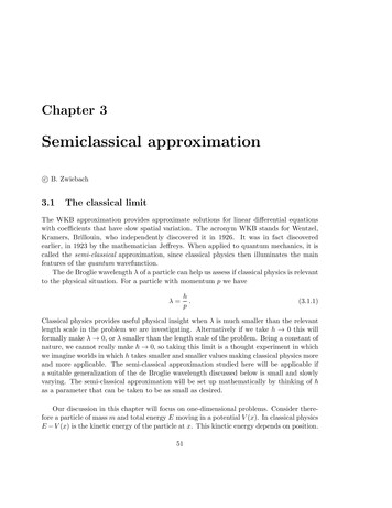
58CHAPTER 3. WKB AND SEMICLASSICAL APPROXIMATIONThis now meansdλ1.dx(3.2.28)The de Broglie wavelength must vary slowly. Note the consistency with units, the left-handside of the inequality being unit free. More intuitive, perhaps, is the version obtained bymultiplying the above by λdλλλ.(3.2.29)dxThis tells us that the variation of the de Broglie wavelength λ over a distance λ must bemuch smaller that λ.It is not hard to figure out what the above constraints tell us about the rate of changeof the potential. Finally connect to the potential. Taking one spatial derivative of theequation p2 2m(E V (x)) we getdVdx pp0 mdV1 pp0 .dxm (3.2.30)Multiplying by the absolute value of λ h/pλ(x)p2dV2π 0 p , dxmm(3.2.31)where the last inequality follows from (3.2.25). Hence, we find thatλ(x)dVdxp2.2m(3.2.32)The change in the potential over a distance equal to the de Broglie wavelength must bemuch smaller than the kinetic energy. This is the precise meaning of a slowly changingpotential in the WKB approximation.The slow variation conditions needed for the basic WKB solutions to be accurate failnear turning points. This could be anticipated since at turning points the local momentumbecomes zero and the de Broglie wavelength becomes infinite. Under general conditions,sufficiently near a turning point the potential V (x) is approximately linear, as shown inFigure 3.1. We then haveV (x) E g(x a) ,g 0.(3.2.33)In the allowed region x a the local momentum isp2 2m((E V (x)) 2mg(a x) .(3.2.34)
3.3. CONNECTION FORMULA59Figure 3.1: The slow-varying conditions in WKB are violated at turning points.As a result, the de Broglie wavelength is given byλ(x) 2π 2π .p2mg a x(3.2.35)π 1 .2mg (a x)3/2(3.2.36)Taking a derivative, we finddλdxThe right-hand side goes to infinity as x a and therefore the key condition (3.2.28) isviolated as we approach turning points. Our basic WKB solutions can be valid only aslong as we remain away from turning points. If we have a turning point, such as x a inthe figure, we need a ‘connection formula’ that tells us how a solution far to the left and asolution far to the right of the turning point are related when they together form a singlesolution. We will consider a connection formula right below.3.3Connection formulaLet us first explain and then use a set of connection formulae, leaving their derivation fornext section. The connection formulae refer to solutions away from a turning point x aseparating a classically allowed region to the left and a classically forbidden region to theright. This is the situation illustrated in Figure 3.2.For such turning point at x a the WKB solutions to the right are exponentials thatgrow or decay and the WKB solutions to the left are oscillatory functions. They connect
60CHAPTER 3. WKB AND SEMICLASSICAL APPROXIMATIONFigure 3.2:consistent with the following relations Z a Z x π120000pcosk(x )dx pexp κ(x )dx4k(x)κ(x)xa1 psink(x) Zxak(x0 )dx0 π4 1 pexpκ(x) Zxκ(x0 )dx0(3.3.1) (3.3.2)aIn the first relation the arrow tells us that if the solution is a pure decaying exponential tothe right of x a the solution to the left of x a is accurately determined and given bythe phase-shifted cosine function the arrow points to. The second relation says that if thesolution to the left of x a is of an oscillatory type, the growing part of the solution tothe right of x a is accurately determined and given by the exponential the arrow pointsto. The decaying part cannot be reliably determined. As we will elaborate upon later, anyconnection formula is not to be used in the direction that goes against the arrow.Example: Find a quantization condition for the energies of bound states in a monotonically increasing potential V (x) that has a hard wall at x 0. Assume V (x) increaseswithout bound, as illustrated in Figure 3.3.Let E denote the energy of our searched-for eigenstate. Clearly, the energy and thepotential V (x) determine the turning point x a. The solution for x a must only have adecaying exponential since the forbidden region extends forever to the right of x a. Thewavefunction for x a is therefore of the type on the right-side of the connection formula(3.3.1). This means that we have an accurate representation of the wavefunction to the leftof x a. Adjusting the arbitrary normalization, we have Z a 100πψ(x) pcosk(x )dx 4 , 0 x a .(3.3.3)k(x)x
3.3. CONNECTION FORMULA61Figure 3.3: A monotonically increasing potential with a hard wall at x 0. For an energy eigenstateof energy E the turning point is at x a.Since we have a hard wall, the wavefunction must vanish for x 0. The condition ψ(0) 0requires thatZ acos 0 , with k(x0 )dx0 π4 .(3.3.4)0This is satisfied whenZ ak(x0 )dx0 0π4π2n Z.(3.3.5)π , n 0, 1, 2, . . . .(3.3.6) nπ ,The quantization condition is thereforeZ0ak(x0 )dx0 n 34 Negative integers are not allowed because the left-hand side is manifestly positive. Theabove is easy to use in practice. Using the expression for k(x) in terms of E and V (x) wehaveZ ar 2m(E V (x0 )) dx0 n 34 π , n 0, 1, 2, . . .(3.3.7)2 0In some special cases a can be calculated in terms of E and the integral can be doneanalytically. More generally, this is done numerically, exploring the value of the integralon the left hand side as a function of E and selecting the energies for which it takes thequantized values on the right-hand side.
62CHAPTER 3. WKB AND SEMICLASSICAL APPROXIMATIONLet us rewrite the wavefunction using Z1Rax a0Ra0 0Rx0:Zπ4ψ(x) pcosk(x )dx k(x)0 Z x100k(x )dx pcos k(x)0 Z x sin 00 psink(x )dx ,k(x)0x0k(x )dx0 0(3.3.8)where we expanded the cosine of a sum of angles and recalled that cos 0. In this formit is manifest that the wavefunction vanishes at x 0. More interestingly, the quantizationcondition (3.3.6) indicates that the excursion of the phase in the solution from 0 to a is abit higher than nπ (but less than (n 1)π). Thus the WKB wavefuntion produces the nnodes the n-th excited state must have, even though this wavefunction is not reliable all toway to x a.3.4Airy functions and connection formulae(3.4.9)V (x) E ' g(x a)with g 0 for x a(3.4.10)SolutionsAψ(x) pκ(x) Zexp x0κ(x )dx0 B Zx00 pexpκ(x )dxκ(x)a Z a Z a CD0000ψ(x) pexp ik(x )dx pexp ik(x )dxk(x)k(x)xxx a(3.4.11)ax a (3.4.12)
3.4. AIRY FUNCTIONS AND CONNECTION FORMULAE63wherek2 2m2mg(E V (x)) ' 2 (a x) 2 2mg2m(V (x) E) ' 2 (x a)2 Idea: Solve Schrodinger equationκ2 x a(3.4.13)x a(3.4.14) 2 00ψ (V (x) E)ψ 02mwith the exact linear potential, i.e. (3.4.15) 2 00ψ g(x a)ψ 02m(3.4.16) Solve (3.4.16) exactly. Match it to the x a version of (3.4.11) or x a version of (3.4.12). Find the required relations between coefficients!Solve (3.4.16). Remove units, find length scale. 2 gL L mL2so define u 2mg 2 2mg 13(3.4.17) 13(x a) η(x a)(3.4.18)thus (3.4.16) becomesd2 ψ uψ 0du2(3.4.19)ψ αAi (u) βBi (u)(3.4.20)with solutionwhere α and β are constants and Ai (u), Bi (u) are Airy functions: 1u 1, 12 1π u 4 e ξAi (u) ' 1 u 41 cos ξ π u 1.4πBi (u) 'with 1 1π u 4 eξ(3.4.21)u 1, 1 u 14 sin ξ π 4π3ξ 32 u 2 .(3.4.22)u 1.(3.4.23)These are in fact WKB solutions and special cases of connection conditions! (Explain)
64CHAPTER 3. WKB AND SEMICLASSICAL APPROXIMATION3.4.1How bad are the errors?Take a WKB solution and find the DE it satisfiesψ(u) 1u3214e 3 u 2(3.4.24)solvesd2 ψ 5 1 u ψ 0du216 u2(3.4.25)so clearly for u 1 the extra term is negligible.To evaluate (3.4.11) and (3.4.12), determine κ(x) and k(x). Using (3.4.13) and (3.4.14):Using0 ddx ,k 2 η 3 (a x) η 2 u η 2 u u 0(3.4.26)κ2 η 3 (x a) η 2 uu 0(3.4.27)the WKB condition is k 0 k 2 From .η3η3η2 2 k 2η u 2 u 2kk 0 η 3 k 0 (3.4.28)k 2 η 2 u thus k 0 k 2 ,3η21η 2 u u 2 u 0.632 u 2(3.4.29)Two integrals to estimatexZx a:00ZaZax a:00Zk(x )dx xxp32 3η 3 (x0 a)dx0 η 2 (x0 a) 23a32 32 32 3 η 2 (x a) 2 u 2 u 2 ξ333κ(x )dx apxη 3 (a x0 )dx0xa(3.4.30) a20 32 η (a x )3x3232 32 3 η 2 (a x) 2 u 2 ξ33(3.4.31)both integrals are equal to ξ.11p 1 1 ,κ(x)η 2 u 411p 1 1k(x)η 2 u 4(3.4.32)
3.4. AIRY FUNCTIONS AND CONNECTION FORMULAE651(3.4.11) and (3.4.12), let {A, B, C, D} η 2 {A, B, C, D} 1π to cancel the extra factor andproduce the . constants11 u 4 u 4ψ(x) A e ξ B eξππ 2AAi (u) BBi (u)1u 1(3.4.33)1 u 4 u 4ψ(x) C eiξ D e iξππu 1(3.4.34)Note that1π u 4Ai iBi e i(ξ 4 )π(3.4.35)1π u 4Ai iBi ei(ξ 4 )π(3.4.36)thus1 u 4e (Ai iBi ) eiξπi π4(3.4.37)1 i π4e u 4(Ai iBi ) e iξπ(3.4.38)Now back in (3.4.34):ππψ(x) Cei 4 (Ai iBi ) De i 4 (Ai iBi ) ππππ Cei 4 De i 4 Ai iDe i 4 iCei 4 Bi(3.4.39)Finally equate (one solution):ππi π4 i π42A Cei 4 De i 4iB Ce De(3.4.40) π1C e i 4 (2A iB)21 iπD e 4 (2A iB)2(3.4.41)(3.4.42)(3.4.43)back in (3.4.12) Z a Z a 1 (2A iB)π1 (2A iB)π0000ppψ(x) exp ik(x )dx exp ik(x )dx 2424k(x)k(x)xx
66CHAPTER 3. WKB AND SEMICLASSICAL APPROXIMATION2Aψ(x) pcosk(x) Zxaπk(x )dx 400 B psink(x) Zxaπk(x )dx 400 (3.4.44)Now discuss a subtlety. The formulas are in reality only usable in one direction with partialresults. Some terminology helps. We always speak having in mind a fixed turning point. Ifwe say we have a growing exponential at a turning point we mean we have a solution thatgrows as we move away from the turning point towards the classically forbidden region.Similarly, a decaying exponential means our solution decays as we move away from theturning point towards the classically forbidden region. In summary the connection arrowcan go from a decaying exponential into an oscillatory solution and can go from an oscillatory solution into a growing exponential.3.4.2The other connection conditionsThis time the turning point is at x b, with the classically allowed region to the right of itand the classically forbidden region to the left of it. Z b Z x200pexp κ(x )dx pcosk(x0 )dx0 κ(x)k(x)xb Z b Z x11 pexpκ(x0 )dx0 psink(x0 )dx0 κ(x)k(x)xb1π4 π4 (3.4.45)(3.4.46)For the first relation, if there is only a decaying exponential to the left, the wavefunctionis definitely without the growing exponential, and the wavefunction to the right of x b isaccurately determined. This does not work in the reverse direction because a small error inthe oscillatory function would give a growing exponential to the left of for x b that wouldovertake the predicted decaying solution.For the second relation, the stated direction (from right to left) is reliable: an smallerror on the right side of x b would produce a decaying exponential, thus a small erroron the left-side of x b. The reverse direction does not work: a small error to the left ofx b, a decaying exponential, would produce a large error in the right-hand side.
3.5. TUNNELLING THROUGH A BARRIER67In summary, in all cases of the connection conditions, relative to a turning point,We can connect away from a decaying exponential and into a growing exponential.(3.4.47)3.5Tunnelling through a barrierFigure 3.4: Tunneling in the WKB approximation. The energy E must be smaller than the heightof the potential, and the barrier must be wide and smooth.We want to find the tunneling probability T for a wave of energy incident on a smoothlyvarying wide barrier. The energy E of the wave must be smaller than the height of thepotential. In this problem there is an incident wave, a reflected wave and a transmittedwave, and the associated WKB expressions will have amplitudes controlled by constantsA, B, and F , respectively. The situation is illustrated in Figure 3.4.Remarks:1) Expect T to be small. Little probability flux goes through and A B .2) For x b there is just an outgoing wave with amplitude controlled by F .3) Within the barrier the component that decays as x grows is more relevant that thecomponent that grows. It is the only component that can be estimated reliably.Consider the transmitted right-moving wave valid for x b Z x Fψtr (x) pexp ik(x0 )dx0 i π4 ,k(x)bx b.(3.5.1)This is a WKB solution with an extra phase of π/4 chosen to make the argument of theexponential have the familiar form appearing in the connection formulae. Expanding the
68CHAPTER 3. WKB AND SEMICLASSICAL APPROXIMATIONexponential ZFψtr (x) pcosk(x)x00k(x )dx bπ4 iF psink(x) Zx00k(x )dx bπ4 , x b . (3.5.2)This is in standard form. We can now match the second term to an exponential that growsas we move to the left of x b, by using (3.4.46)ψ(x)barriF pexpκ(x) Zb0κ(x )dx0 , a x b.(3.5.3)xThe subscript ‘barr’ indicates a solution in the barrier region. If we attempted to matchthe first term in (3.5.2) we would get an exponential that decays as we move to the left ofx b and it is unreliable given the growing exponential. We can now refer this solution tothe point x a Z b Z xiF0000ψ(x)barr pexpκ(x )dx κ(x )dxa x b.(3.5.4)κ(x)aaDefiningZθ bκ(x0 )dx0(3.5.5)awe haveψ(x)barr Z x iF eθ00 pexp κ(x )dxκ(x)aa x b.(3.5.6)Since this is a decaying exponential to the right of x a we can connect it to a solution tothe left of x a using (3.3.1) Z a 2iF eθ00πcosk(x )dx 4 .(3.5.7)ψ(x) pk(x)xThis is a superposition of two waves, a wave ψinc incident on the barrier and a wave ψrefreflected from the barrier. The incident part is Z a iF eθ00πψinc (x) pexp ik(x )dx i 4 .(3.5.8)k(x)xThe sign in front of the integral may seem unusual for a wave moving to the right, butit is correct because the argument x appears in the lower limit of the integration. Thetransmission coefficient T is the ratio of the transmitted probability current over the incidentprobability current. Given the result in (3.2.19) we haveT F 2probability current for ψtr e 2θ .probability current for ψinc iF eθ 2(3.5.9)
3.5. TUNNELLING THROUGH A BARRIER69This is the well-known exponential suppression of the transmission coefficient. Using theearlier definition of θ the result is Z b Twkb exp 2κ(x0 )dx0 .(3.5.10)aWe added the subscript ‘wkb’ to emphasize that this is the WKB approximation to theexact transmission coefficient. The integral extends in between the two turning points andcaptures information about the height and the width of the barrier. The integrand, as wellas the turning points, depend on the energy as we can display by using the explicit valueof κ(x) : Z b r 2m 0 ) E) dx0 .Twkb exp 2(V(x(3.5.11) 2aThe WKB approximation only captures the exponentially decaying part of the transmissioncoefficient. There are corrections that are written as a prefactor to the exponential. Theseare not determined in this approximation.Example. Use the WKB approximation to estimate the transmission probability T for therectangular barrier(V0 for x a ,V (x) (3.5.12)0 , otherwise.Assume the barrier is large. In terms of the familiar unit-free constant z0 used to characterizesquare wells, this means that2mV0 a2z02 1.(3.5.13) 2Large barrier means large z0 or large V0 a2 . Moreover we assume E smaller than V0 ; wecannot expect the approximation to work as the energy approaches the top of the barrier.Compare the WKB result for T with the exact result.Solution. The WKB estimation, using (3.5.11) is immediate. Since the barrier extendsfrom x a to x a and the potential is constant we have Z a r 2m0Twkb exp 2(V E)dx.(3.5.14)0 2 aThe integral can be done and we findTwkb 4a p exp 2m(V0 E) . This is the answer in the WKB approximation. In terms of z0 this readsr E Twkb ' exp 4z0 1 .V0(3.5.15)(3.5.16)
70CHAPTER 3. WKB AND SEMICLASSICAL APPROXIMATIONThe validity of the WKB approximation requires the argument in the exponent to be large.This is why we need z0 1 and the energy not to approach V0 . When E is very smallcompared to V0 , we haveT exp( 4z0 ) .(3.5.17) Since z0 a V0 , this result is the basis for the claim that the exponential suppression ofthe tunneling probability is proportional to the width of the well and the square root of itsheight.The exact formula for the tunneling probability of a square barrier has been calculatedbefore, and it is given by 2a p 1V02 1 sinh22m(V0 E) .T4E(V0 E) (3.5.18)This formula will allow us to confirm the WKB exponential suppression and to find theprefactor. Under the conditions z0 1 and V0 E finite, the argument of the sinh functionis large so this function can be replaced by its growing exponential (sinh x 12 ex ):1V0' 1 T16E(1 EV0 )exp 4a p2m(V0 E) , (3.5.19)where we also replaced V0 E V0 in the prefactor. The additive unit on the right-handside can be neglected and we haveT ' 16 VE0 (1 EV0 ) 4a p exp 2m(V0 E) . (3.5.20)This result gives the same in exponential suppression as the WKB result (3.5.15). It alsogives us a good approximation to the prefactor.The WKB approximation is often used for the estimation of lifetimes. The physicalsituation is represented in Figure 3.5. We have a particle of mass m and energy E localizedbetween the turning points x a and x b of the potential. The classical particle cannotescape because of the energy barrier stretching from x b to x c. The quantum particle,however, can tunnel. The state of the quantum particle when localized between a and bis not strictly an energy eigenstate be
The de Broglie wavelength of a particle can help us assess if classical physics is relevant to the physical situation. For a particle with momentum pwe have h p: (3.1.1) Classical physics provides useful physical insight when is much smaller than the relevant length scale in the problem we