Transcription
Chapter 1Angular Momentum in QuantumMechanics1.11.1.1Classical vectors vs quantum operatorsRelevant definitions and notationIn classical physics, the angular momentum L of a particle is given by the cross product ofits position vector r and momentum vector p:L r p.(1.1)In quantum physics, we can construct an analogous operator by defining the ”vector” operators r̂ and p̂ as follows:r̂ x̂1 e1 x̂2 e2 x̂3 e3(1.2)p̂ p̂1 e1 p̂2 e2 p̂3 e3where i 1, 2, 3 correspond to x, y, z, resp., and the ei are ortho-normal unit vectors in the3-dimensional vector space. The ”hat” (ˆ) symbols signify that these are operators, and thebold type signifies that it is a construction of operators with unit vectors, which we will referto as vector operators. This notation allows us to perform the classical vector operations,such as dot- and cross-products. In particular, by maintaining the classical equation for theangular momentum vector, we are able to write the L̂i component of the angular momentumoperator given in Eq. 1.1 in the following way:L̂1 x̂2 p̂3L̂2 x̂3 p̂1L̂3 x̂1 p̂2x̂3 p̂2x̂1 p̂3x̂2 p̂1(1.3)and the orbital angular momentum vector operator is L̂ L̂1 e1 L̂2 e2 L̂3 e3 .Eq. 1.3 can be more compactly written as:L̂i "ijk x̂j p̂k5(1.4)
6CHAPTER 1. ANGULAR MOMENTUM IN QUANTUM MECHANICSwhere "ijk is the three-dimensional Levi-Civita symbol, and we employ the Einstein summation convention, i.e. repeated indices imply a sum over that index. This notation will beused in other parts of these notes.1.1.2Quantum vector operationsIn order to build up a formalism using our quantum vector operators, we need to examinesome of their important properties. While the classical position and momentum xi and picommute, this is not the case in quantum mechanics. The commutation relations betweenposition and momentum operators is given by:[x̂i , x̂j ] 0,[p̂i , p̂j ] 0,[x̂i , p̂j ] i ij ,(1.5)where ij is the Kronecker delta symbol. It should be noted that the ei unit vectors commutewith all operators.To see how the vector operators behave under dot and cross products, we can apply themin the normal way:û · v̂ ûi v̂i(1.6)(û v̂)i "ijk ûj v̂kUnlike with classical vectors, these are operators, and their order can, in general, not bechanged. For the case of the dot-product, switching the order of the vector operators resultsin:û · v̂ [ûi , v̂i ] v̂i ûi(1.7) v̂ · û [ûi , v̂i ]Contrast this with the classical dot product result, where u · v v · u. It is now clear thatthe classical result holds true for commuting operators, but not in the general case wherethe operators may not commute. Note the special case of û2 û · û, which does obey theclassical dot product relationship.Similarly, the cross product can we written as:(û v̂)i "ijk ([ûj , vˆk ] v̂k ûj ) "ikj v̂k ûj "ijk [ûj , vˆk ] (v̂ û)i "ijk [ûj , v̂k ]which, again, contrasts with the classical result u v operators.(1.8)v u in the case of non-commutingIf we look at the special cases r̂ r̂ and p̂ p̂ we see that:1(r̂ r̂)i (p̂ p̂)i "ijk2jk 0where the last equality is obvious due to the contradictory requirements of "ijk andbe non-zero.(1.9)jkto
1.1. CLASSICAL VECTORS VS QUANTUM OPERATORS7In the case where û r̂ and v̂ p̂, Eq. 1.7 and Eq. 1.8 result in:r̂ · p̂ p̂ · r̂ 3i r̂ p̂ p̂ r̂(1.10)The cross product between r̂ and p̂ obeys classical rules, however the dot product does not.1.1.3Properties of angular momentumA simple analysis can be done to show:(û · v̂)† v̂ † · û†(û v̂)† v̂ † û†(1.11)This property can be used to show that L̂ is Hermitian (given that r̂ and p̂ are Hermitian):L̂† (r̂ p̂)† p̂ r̂ L̂.(1.12)It is simple to determine that L̂ is orthogonal to both r̂ and p̂, just as it is classically:r̂ · L̂ p̂ · L̂ x̂i L̂i ,"ijk x̂i x̂j p̂k 0,p̂i L̂i ,"ijk p̂i x̂j p̂k 0.(1.13)The last step of each equation is true due to the sign change of "ijk under a swap of indices,and the commutation properties of position and momentum operators.To see how angular momentum commutes with position or momentum, we can use Eq. 1.4to write:[L̂i , x̂j ] "ikl x̂k p̂l x̂j "ikl x̂j x̂k p̂l "ikl {x̂k (x̂j p̂l i jl ) x̂j x̂k p̂l }(1.14) i "ikj x̂k "ikl (x̂k x̂j p̂l x̂j x̂k p̂l ) i "ijk x̂kThe treatment for momentum is very similar, and in summary we obtain the equations:[L̂i , x̂j ] i "ijk x̂k[L̂i , p̂j ] i "ijk p̂k(1.15)These equations are said to mean that r̂ and p̂ are vectors under rotations.Using Eq. 1.15 it is possible to derive the commutation relations between di erent components of L̂:[L̂i , L̂j ] L̂i "jkl x̂k p̂l "jkl x̂k p̂l L̂i"jkl (x̂k L̂i i "iku x̂u )p̂l "ikl x̂k p̂l L̂ii "jkl "iku x̂u p̂l "jkl x̂k (p̂l L̂i i "ilv p̂v ) "ikl x̂k p̂l L̂ii ("kjl "kiu x̂u p̂l "lkj "liv x̂k p̂v )i [( ij luil ju )x̂u p̂l ( ik jvij kv )x̂k p̂v ]i ( ij x̂l p̂l x̂j p̂i x̂i p̂jx̂p̂)ij k ki (x̂i p̂j x̂j p̂i )(1.16)
8CHAPTER 1. ANGULAR MOMENTUM IN QUANTUM MECHANICSwhere in the fourth step we made use of the identity "ijk "ilm jl kmjm kl .We can write the result in Eq. 1.16 explicitly as:[L̂x , L̂y ] i L̂z ,[L̂y , L̂z ] i L̂x ,[L̂z , L̂x ] i L̂y ,(1.17)and which can be compactly written as:[L̂i , L̂j ] i "ijk L̂k .(1.18)It is now clear that di erent components of the angular momentum do not commute. Wecan additionally use Eq. 1.18 to straightforwardly show that:[L̂i , r̂ 2 ] 0,[L̂i , p̂2 ] 0,, [p̂i , r̂ · p̂] 0,, [L̂i , L̂2 ] 0,(1.19)where in particular the last equation (for L̂2 ) is important. Even though L̂i does not commutewith any other component of L̂, it does commute with L̂2 .There is a more elegant way to express the algebra of angular momentum. Using Eq. 1.8and Eq. 1.18 we can write(L̂ L̂)i (L̂ L̂)i "ijk [L̂j , L̂k ]i 2 "jki "jkm L̂m , i 2 ( kk imkm ik )L̂m ,i 2 (L̂iik L̂k ), i L̂i ,(1.20)L̂ L̂ i L̂.(1.21)or, in shortThis result gives an intuitive feel for why angular momentum behaves in an inherentlyquantum way. A non-zero cross product of a vector with itself is contrary to any classicalphenomenom. It is also important to note that, since we only used the general mathematicalproperties of the cross product of quantum vectors, and the commutation relations of angularmomentum operators, Eq. 1.18 and Eq. 1.21 are completely equivalent to each other.1.2Angular momentum and central potentialsWe now consider the orbital angularp momentum in the context of central potentials (potentials that depend only on r r̂ 2 ), such as the Coulomb potential of an electron in theelectric field of an atomic nucleus. The Hamiltonian in this case is given byĤ p̂2 V (r),2mr pr̂ 2 .(1.22)
1.3. ALGEBRA OF ANGULAR MOMENTUM9We can write this Hamiltonian in position space using p̂ i r, or p̂2 r2 is the Laplace operator. In spherical coordinates, this is 211 @@1 @222 1 @p̂ r 2sin r @r2rsin @ @ sin2 @ 2 2 r2 , where(1.23)We can write L̂2 in spherical coordinates as follows:L̂2 2 (r̂ h r) · (r̂ r) i h i1 @2 ˆ sin @ ˆ @@ · ˆ sin1 @@ ˆ @@hh 2i 2 ˆ i ˆ@@ ˆ @@ ˆ1 @ ˆ @ ˆ @2ˆˆˆˆ@2@ @ sin2 @ 2 @ @ @ sin @ sin @ @ @ @ @ 1@2cos @@22 sin2 @ 2 sin @ @ 2 2@@ 2 sin1 @ sin @ sin12 @@ 2(1.24)Note that the angular momentum has no r-dependence.Using Eq. 1.24 and Eq. 1.23, we can rewrite the Hamiltonian as:Ĥ 2 @ 2L̂2r V (r)2mr @r22mr2(1.25)We can now assemble a list of Hermitian operators (observables) we have discussed:Ĥ,x̂1 ,x̂2 ,x̂3 ,p̂1 ,p̂2 ,p̂3 ,r̂ 2 ,p̂2 ,L̂1 ,L̂2 ,L̂3 ,L̂2(1.26)where we include all unique Hermitian operators that include up to squared terms of positionor momentum.Typically in atomic physics, the spectrum (energy levels) of an atom is of major interest.We therefore want to only consider observables that commute with the Hamiltonian. Thisexcludes the x̂i operators (don’t commute with p̂2 ) and p̂i operators (don’t commute withV (r), in general). The same reasoning eliminates r̂ 2 and p̂2 . However, from Eq. 1.25 it isclear that the L̂i operators and L̂2 commute with H. Due to the L̂i not commuting witheach other, we can only use one of them in our set of operators. The convention for this isL̂z . Our set of commuting Hermitian operators (observables) is then:Ĥ,1.3L̂z ,L̂2(1.27)Algebra of angular momentumHermitian operators Jˆx , Jˆy , and Jˆz are said to satisfy the algebra of angular momentum ifthey obey the commutation relations given by Eq. 1.18:[Jˆi , Jˆj ] i "ijk Jˆk .(1.28)
10CHAPTER 1. ANGULAR MOMENTUM IN QUANTUM MECHANICSKeep in mind that this could be orbital angular momentum L̂i , spin angular momentum Ŝi ,or any other set of Hermitian operators that obeys the above commutation relation. As weshowed in section 1.1.3, from this algebra it also follows that:[Jˆi , Jˆ2 ] 0.(1.29)Jˆ Jˆx iJˆy .(1.30)Define then the following operators:Note that these operators are each other’s Hermitian conjugate Jˆ † Jˆ .To understand the behavior of these operators and how they act on the angular momentumoperators, we can do some simple manipulations:Jˆ Jˆ Jˆx2 Jˆy2 i[Jˆx , Jˆy ] Jˆx2 Jˆy2 Jˆz ,and so the commutator is[Jˆ , Jˆ ] 2 Jˆz .(1.31)(1.32)In addition, we can see the following are all equal:Jˆ2Jˆz2 Jˆx2 Jˆy2 Jˆ Jˆ1 ˆ ˆ(J J Jˆ Jˆ ) Jˆz Jˆ Jˆ Jˆz 2(1.33)Since we also know that the individual components commute with Jˆ2 we know that the samemust be true for Jˆ :[Jˆ , Jˆ2 ] 0.(1.34)Lastly, we calculate the commutation with Jˆz :[Jˆz , Jˆ ] [Jˆz , Jˆx ] i[Jˆz , Jˆy ] i Jˆy i( i )Jˆx Jˆ (1.35)Since each Jˆi and Jˆ2 commute, we can simultaneously diagonalize them. However, thedi erent Jˆi do not commute with each other, so we have to choose one. Typically, this is Jˆz .The simultaneous eigenstates are denoted by j, mi, and they form an orthonormal basis. Sofar, the only restriction on j and m is j, m 2 R.We label the states in such a way that the following relations apply:Jˆ2 j, mi 2 j(j 1) j, miJˆz j, mi m j, mi(1.36)The reason why we choose to define the values using j(j 1) (as opposed to j 2 ) is for futurealgebraic convenience, as we will see.
1.3. ALGEBRA OF ANGULAR MOMENTUM11Since it is a requirement that j(j 1)0, it is necessary that either j 1 pr jHowever, since the only thing that matters is the eigenvalue, we can just choose j 0.0.To see how the operators Jˆ act on j, mi we will check the eigenvalue of Jˆ2 after acting ona state:Jˆ2 (Jˆ j, mi) Jˆ Jˆ2 j, mi 2 j(j 1)(Jˆ j, mi).(1.37)2From this it is clear that Jˆ is still an eigenstate of Jˆ while keeping the eigenvalue junchanged. However, it is still unknown if it changes the m eigenvalue. To investigate this,we follow the same procedure, but with Jˆz :Jˆz (Jˆ j, mi) (Jˆ Jˆz Jˆ ) j, mi (m 1)(Jˆ j, mi).(1.38)We see that the m eigenvalue is increased (decreased) by 1 when acted on by Jˆ (Jˆ ).Putting together Eq. 1.37 and Eq. 1.38 we can state:Jˆ j, mi C (j, m) j, m 1i(1.39)where C (j, m) can be determined by taking the inner product of Eq. 1.39 with its Hermitianconjugate:hj, m 1 C (j, m)C (j, m) j, m 1i C (j, m) 2 ,hj, m Jˆ Jˆ j, mi ,hj, m Jˆ2 Jˆz2 Jˆz j, mi , 2 [j(j 1) m(m 1)].(1.40)This equation shows the convenience of using j(j 1) as the eigenvalue of Jˆ2 . While thisequation is simple, we can use it to determine many things about our vector space. For onething, since C (j, m) 2 is the norm of a vector, it must be non-negative, i.e. we must havej(j 1) m(m 1) 0. We can analyze the and - cases separately.( )( )j(j 1)j(j 1)m(m 1)m(m 1)00 ) )j 1 m j,j m j 1.(1.41)These conditions need to both be true at all times, and so we must use the strictest conditions:j m j.(1.42)So far there are no requirements on j. However, let’s consider a state less than one unitbelow the maximum value of m, i.e. j, m ki for some 0 k 1. Acting on this statewith Jˆ gives us a state j, m k 1i that is inconsistent with the requirements in Eq. 1.42.The only way to resolve this issue is to ensure that when Jˆ acts on the upper state weobtain the null state, i.e. C (j, m) 0. This condition is satisfied when m j. Similarly,C (j, m) 0 when m j. This also means that there need to be an integer number ofsteps to get from m j to m j, and therefore:2j 2 N!j 2 N/2!j 2 0, 12 , 1, 23 , 2, 52 , .m 2 { j, j 1, j 2, ., j2, j(1.43)1, j}These are the fundamental quantization properties of angular momentum. They hold fororbital angular momentum, spin angular momentum, and any other space in which Eq. 1.28is satisfied.
In classical physics, the angular momentum L of a particle is given by the cross product of its position vector r and momentum vector p: L r p. (1.1) In quantum physics, we can construct an analogous operator by defining the ”vector” oper-ators rˆ and pˆ as follows: rˆ ˆx 1e 1 ˆx 2e 2 ˆx 3e 3 pˆ ˆp 1e 1 ˆp 2e 2 ˆp 3e 3 (1.2) where i 1,2,3correspondtox,y,z,resp .