Transcription
Ecological Economics 57 (2006) 534 – l and monetary input–output analysis:What makes the difference?Helga Weisz a,*, Faye Duchin baInstitute of Social Ecology, Faculty of Interdisciplinary Studies (IFF), Klagenfurt University, Vienna, Schottenfeldgasse 29,1070 Vienna, AustriabDepartment of Economics, Rensselaer Polytechnic Institute, 110 8th St., Troy, NY 12180, USAReceived 30 November 2004; received in revised form 8 May 2005; accepted 9 May 2005Available online 6 July 2005AbstractA recent paper in which embodied land appropriation of exports was calculated using a physical input–output model(Ecological Economics 44 (2003) 137–151) initiated a discussion in this journal concerning the conceptual differences betweeninput–output models using a coefficient matrix based on physical input–output tables (PIOTs) in a single unit of mass andinput–output models using a coefficient matrix based on monetary input–output tables (MIOTs) extended by a coefficient vectorof physical factor inputs per unit of output. In this contribution we argue that the conceptual core of the discrepancies foundwhen comparing outcomes obtained using physical vs. monetary input–output models lies in the assumptions regarding unitprices and not in the treatment of waste as has been claimed (Ecological Economics 48 (2004) 9–17). We first show that a basicstatic input–output model with the coefficient matrix derived from a monetary input–output table is equivalent to one where thecoefficient matrix is derived from an input–output table in physical units provided that the assumption of unique sectoral pricesis satisfied. We then illustrate that the input–output tables that were used in the original publication do not satisfy theassumption of homogenous sectoral prices, even after the inconsistent treatment of waste in the PIOT is corrected. We showthat substantially different results from the physical and the monetary models in fact remain. Finally, we identify and discusspossible reasons for the observed differences in sectoral prices faced by different purchasing sectors and draw conclusions forthe future development of applied physical input–output analysis.D 2005 Elsevier B.V. All rights reserved.Keywords: Physical input–output analysis; Monetary input–output analysis; MIOT; PIOT; Total physical resource requirements; Sectoral unitprices1. Introduction* Corresponding author. Tel.: 43 1 522 40 00 410; fax: 43 1522 40 00 477.E-mail address: helga.weisz@uni-klu.ac.at (H. Weisz).0921-8009/ - see front matter D 2005 Elsevier B.V. All rights y, a series of publications in this journalanalyzed the use of input–output models based oncoefficient matrices derived from input–output tables
H. Weisz, F. Duchin / Ecological Economics 57 (2006) 534–541in mass units (PIOTs) for the computation of directand indirect physical factor requirements to satisfy agiven bill of final deliveries and compared them toinput–output models using coefficient matrices derived from monetary tables (MIOTs) and a vector ofphysical factor inputs per unit of output.Hubacek and Giljum (2003) claimed that physicalinput–output models are more appropriate to accountfor direct and indirect resource requirements (such asland area, raw materials, energy, or water). In theirpaper the authors computed direct and indirect landattributable to exports. They compared two models,one using a coefficient matrix based on a monetarytable and the other using a coefficient matrix based on aphysical table (both tables for Germany (Stahmer et al.,1998), highly aggregated to 3 3) and arrived at substantially different numerical results concerning overalland sectoral land appropriation for exports (see Hubacek and Giljum, 2003, Table 3). The authors concluded:bFor the quantification of direct and indirect resourcerequirements, we, therefore, suggest applying input–output analysis based on PIOTs, as (a) the most material-intensive sectors are also the sectors with the highest land appropriation and (b) physical input–outputanalysis illustrates land appropriation in relation to thematerial flows of each the sectors, which is moreappropriate from the point of view of environmentalpressures than the land appropriation in relation tomonetary flows of a MIOTQ (Hubacek and Giljum,2003, p 146).In a reply to this paper Suh (2004) demonstratedthat waste is misspecified in the PIOT used by Hubacek and Giljum. Suh showed that this misspecificationmakes the PIOT inconsistent in terms of mass balanceand as a consequence is a flawed physical model.Furthermore, it violates the fundamental assumptionof input–output economics that each sector produces ahomogeneous characteristic output (Suh, 2004, pp11). Suh proposed two alternative physical models(denoted as approach 1 and 2), which make use ofPIOTs that consistently apply the mass balanceassumptions and comply with standard assumptionsof input–output analysis (Suh, 2004, Table 3, p 14).Re-calculating Hubacek and Giljum’s original estimate of land appropriation of exports with the twoalternative physical models, Suh arrived at quite different results from Hubacek and Giljum (Suh, 2004,Fig. 1, p15).535Suh determined that major differences in the resultsobtained with physical IO models and an extendedmonetary model are actually due to differences in thetreatment of waste in the PIOT and not to a superiorityof the physical model. He concludes: bThese differences have nothing to do with the dresemblance withphysical realitiesT of PIOTs, as the results from a consistent PIOT approach may be similar to that of a MIOTapproach. Nor does it prove the superiority of thephysical table over the monetary tableQ (Suh, 2004,p14). According to Suh, the differences between amonetary and a physical model may be relativelysmall if the treatment of waste is consistent in termsof mass balance and the underlying assumptions reasonably reflect real world conditions, two criteriawhich, according to Suh, apply to his approach 1.Here we argue that the basic reason for both the largediscrepancies found by Hubacek and Giljum (2003),and the smaller ones found by Suh (2004) when comparing physical and monetary input–output models, isthat both the MIOT and the PIOT they used contradictthe assumption of a unique price for the characteristicoutput of a given industry. We first show that a basicstatic input–output model using a coefficient matrixderived from a monetary input–output table is strictlyequivalent to one where the coefficient matrix derivedfrom an input–output table in physical units providedthat the assumption of unique sectoral prices is satisfied. We then illustrate that neither the models (physicaland monetary) used by Hubacek and Giljum (2003) northe models proposed by Suh (2004) meet the assumption of homogenous sectoral prices and that in generalsingle mass unit physical models deliver substantiallydifferent outcomes as compared to a monetary modelfor this reason. Finally, we identify and discuss possiblereasons for the observed differences in sectoral pricesand draw conclusions for the future development ofapplied physical input–output analysis.2. The conceptual relation between a physical anda monetary modelThe objective of this Section is to demonstrate theequivalence between a basic input–output model withthe variables measured in physical units and one withvariables measured in money units on the assumptionof a unique unit price for the characteristic output of
536H. Weisz, F. Duchin / Ecological Economics 57 (2006) 534–541each sector, as was shown in 1965 by Fisher whodemonstrated that the Leontief system is not sensitiveto a change of units (Fisher, 1965).1To see this we start from the basic input–outputequation:y ¼ ð I AÞxð1Þwhere y is an n 1 vector of final deliveries and x isan n 1 vector of sectoral output, both measured inarbitrary physical units, in this case all output beingmeasured in tons, and A is the n n matrix of coefficients of inputs per unit of output (tons per ton).Let p be the n 1 vector of unit prices (price perton). Pre-multiply both sides of (1) by p̂ and furtherpre-multiply x in the righthand side by I [p̂ p̂ 1],where p̂ is the n n diagonal matrix with the pricevector down the diagonal and p̂ 1 is the n n diagonal matrix with the inverse of the unit prices downthe diagonal. This operation yields: 1 pˆy ¼ p̂p ð I AÞ p̂p p̂p xð2ÞIn other words, the element-by-element divisionof a column of the flow table in monetary units bythe corresponding column in physical units mustyield the n-vector p of unit prices, {p j}. The 2models are the same except for the change of unitoperation, and the vector of unit prices provides theinformation needed for the change of unit.This proof holds in the case of a single physicalunit, as in a PIOT, or in the more general case ofmixed physical units.It follows that a basic input–output model with thecoefficient matrix based on a monetary input–outputtable conceptually must deliver exactly the same resultas a basic input–output model where the coefficientmatrix is based on a physical input–output table if thesame assumptions are made about each sector’s factorrequirements.3. The empirical differences found by Hubacek andGiljum (2003) and by Suh (2004)or pˆy ¼ pp̂ ð I AÞp̂p 1 p̂pxwhere p̂y is the n 1 vector of final deliveries inmonetary values, p̂ (I A) p̂ 1 is the n n coefficientmatrix in money values, and p̂x is the n 1 vector ofoutputs in money values. Thus if (1) holds in physicalunits, then (2) holds in money units, and the converseis also easily demonstrated.Note that if the coefficient matrices are derivedfrom flow tables, the relationship between the tablein physical units and that in monetary units can beformalized as follows. Let Z p be the n n table offlows in physical units (in mixed units or, in this case,with all units in tons) and Z m, the n n table of flowsin monetary values. Then an element of Z p is:n o X zji þ yjð3Þzpij ¼ aij xj ; where xj ¼and an element of Zm is: n o 1pj x jzmap¼pjijijj1j ¼ pj aij xjWe now turn to the empirical example provided byHubacek and Giljum (2003) and discussed by Suh(2004). Suh showed that the treatment of waste inHubacek and Giljum’s PIOT was inconsistent due toan inappropriate allocation of production waste in thePIOT because the wastes generated by each sectorwere added to its final deliveries in proportion to itsuse of primary inputs. As Suh rightly argued, theassumption of homogenous products is violated bycombining production waste with commodity deliveries, and the mass balance principle is violated byallocating the production waste in proportion to primary inputs (Suh, 2004). We agree with this assessment but not with Suh’s claims that bthe majordifferences in the results between the approaches aredue mostly to the different principles in treatingwasteQ and that bthe pure difference between thePIOT [if handled consistently] and MIOT is relativelysmallQ (Suh, 2004, p14).2ð4ÞWe thank Sangwon Suh for making us aware of this reference.2The waste problem, important as it, is has been clearlyprivileged so far in the debate on physical and monetary input–output analysis. In contrast to this the role of prices althoughmentioned frequently (see Suh, 2004; Giljum et al., 2004; Dietzenbacher, in press; and Giljum and Hubacek, 2004) has not been fullyrecognized in its relevance.
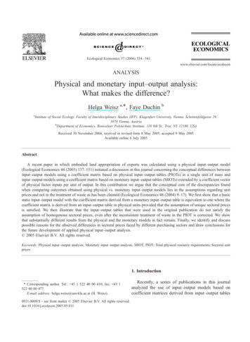
H. Weisz, F. Duchin / Ecological Economics 57 (2006) 534–541Table 1Implicit sectoral prices of commodity outputs in DM per ton,Germany 070.843.805.395.3145.71163.095.67Source: calculated from aggregated MIOT and PIOT for Germanyin 1990 (Stahmer, 2000), as aggregated by Hubacek and Giljum(2003).Instead, we argue that the conceptual root of thedifferences in outcomes is explained by the fact thatthe two models are related by a price matrix ratherthan a price vector. That is, different unit prices arebeing assumed for different purchasers of a givensector’s output. Our claim is demonstrated by a closerexamination of the two tables.The price structure that relates the two input–output tables is readily derived by dividing eachentry in the inter-industry and final demand tables537of the MIOT by the corresponding entry of the PIOT(see Table 1). It is immediately evident that theimplicit sectoral prices vary significantly. In theprimary sector implicit prices vary by a factor of13.6, in the secondary sector by a factor of 6, and inthe tertiary sector by a factor of 30.7. Given theseprice assumptions, even a consistent treatment ofwaste cannot assure comparable results from thetwo models. On the contrary, we must anticipatethat the results from Suh’s (2004) physical modelwill differ substantially from the results of the monetary model.Why then did Suh (2004), unlike Hubacek andGiljum (2003), arrive at similar although not identicalresults for total land requirements of exports using hisphysical model (approach 1) and the extended monetary model? We claim that the similarity between thetwo results gained by Suh is coincidental. This isillustrated in Fig. 1, where we show the direct andindirect land appropriation gained from the monetarymodel and the physical model, not only for exports, asSuh did, but also for domestic final demand. We usedthe same numerical figures as Hubacek and Giljum(2003) and the physical model (approach 1) proposedby Suh (2004).total land approriation (Million ha)20181614121086420PIOT (Suhsapproach 1)MIOTPIOT (Suhsapproach 1)exportsprimary sectorMIOTdomestic FDsecondary sectortertiary sectorFig. 1. Total (direct and indirect) land appropriation for exports and for domestic final demand. Source: aggregated MIOT and PIOT Germany1990 (Stahmer, 2000), aggregation Hubacek and Giljum (2003), land use vector Hubacek an
operation, and the vector of unit prices provides the information needed for the change of unit. This proof holds in the case of a single physical unit, as in a PIOT, or in the more general case of mixed physical units. It follows that a basic input–output model with the coefficient matrix based on a monetary