WIXLIB

ℒ!"# %CNNℒ&# ()*ℒ##StronglyaugmentedHigh-DLoss functionShared weightsSubspace projectionInterpolated embeddingClass prototype“Wolf”Low-Dℒ!"# %normalizeInterpolated 0.2 Input 0.8 Figure 2. Our proposed framework for noise-robust contrastive learning. We project images into a low-dimensional subspace, and regularizethe geometric structure of the subspace with (1)Lcc : a consistency contrastive loss which enforces images with perturbations to have similarembeddings; (2)Lpc mix : a prototypical contrastive loss augmented with mixup, which encourages the embedding for a linearly-interpolatedinput to have the same linear relationship w.r.t the class prototypes. The low-dimensional embeddings are also trained to reconstruct thehigh-dimensional features, which preserves the learned information and regularizes the classifier.contrastive loss maximizes the inner product between thepair of positive embeddings ẑ i and ẑ j(i) , while minimizingthe inner product between 2(b 1) pairs of negative embeddings. By mapping different views (augmentations) of thesame image to neighboring embeddings, the consistency contrastive loss encourages the network to learn discriminativerepresentation that is robust to low-level image corruption.Weakly-supervised mixup prototypical contrastive loss.Our second contrastive loss injects structural knowledge ofclasses into the embedding space. Let Ic denote indices forthe subset of images in D labeled with class c, we calculatethe class prototype as the normalized mean embedding:\Vec {z} c \frac {1}{ \mathcal {I} c } \sum {i \in \mathcal {I} c} \Vec {\hat {z}} i, \Vec {\hat {z}} c \frac { \Vec {z} c}{\left \lVert \Vec {z} c \right \rVert 2},(2)where ẑ i is the embedding of a center-cropped image, andthe class prototypes are calculated at the beginning of eachepoch.The prototypical contrastive loss enforces an image embedding ẑ i to be more similar to its corresponding classprototype ẑ yi , in contrast to other class prototypes:\mathcal {L} \mathrm {pc} (\Vec {\hat {z}} i, y i) -\log \frac {\exp (\Vec {\hat {z}} i\cdot \Vec {\hat {z}} {y i}/\tau )}{\sum {c 1} {C} \exp (\Vec {\hat {z}} i\cdot \Vec {\hat {z}} c/\tau ) }.(3)Since the label yi is noisy, we would like to regularize theencoder from memorizing training labels. Mixup [44] hasbeen shown to be an effective method against label noise [1,18]. Inspired by it, we create virtual training samples bylinearly interpolating a sample (indexed by i) with anothersample (indexed by m(i)) randomly chosen from the sameminibatch:\Vec {x} i m \lambda \Vec {x} i (1-\lambda ) \Vec {x} {m(i)},(4)where λ Beta(α, α).mLet ẑ mi be the normalized embedding for xi , the mixupversion of the prototypical contrastive loss is defined as aweighted combination of the two Lpc w.r.t class yi and ym(i) .It enforces the embedding for the interpolated input to havethe same linear relationship w.r.t. the class prototypes.\mathcal {L} \mathrm {pc\ mix} \sum {i 1} {2b} \lambda \mathcal {L} \mathrm {pc} (\Vec {\hat {z}} i m,y i) (1-\lambda ) \mathcal {L} \mathrm {pc} (\Vec {\hat {z}} i m,y {m(i)}).(5)Reconstruction loss. We also train a linear decoder Wdto reconstruct the high-dimensional feature v i based on z i .The reconstruction loss is defined as:\mathcal {L} \mathrm {recon} \sum {i 1} {2b} \left \lVert \Vec {v} i - \Vec {\mathrm {W}} \mathrm {d} \Vec {z} i \right \rVert 2 2.(6)There are several benefits for training the autoencoder.First, an optimal linear autoencoder will project v i into itslow-dimensional principal subspace and can be understoodas applying PCA [2]. Thus the low-dimensional representation z i is intrinsically robust to input noise. Second, minimizing the reconstruction error is maximizing a lower boundof the mutual information between v i and z i [37]. Therefore,knowledge learned from the proposed contrastive losses canbe maximally preserved in the high-dimensional representation, which helps regularize the classifier.9487

858075700204060EpochCIFAR-10CIFAR-10080 10090807060500204060EpochCIFAR-10CIFAR-10080 100(b)(a)Supervised Noise Ratio (%)90Num. of Sup. Samples (%)Pseudo Label Accuracy c)Figure 3. Curriculum learned by the proposed label correction method for training on CIFAR datasets with 50% sym. noise. (a) Accuracyof pseudo-labels w.r.t to clean training labels. Our method effectively cleans a majority of the label noise. (b) Number of samples in thetweakly-supervised subset Dws. As the pseudo-labels become more accurate, more samples are used to compute the supervised losses. (c)Label noise ratio in the weakly-supervised subset, which maintains at a low level even as the size of the subset grows.Classification loss. Given the softmax output from the classifier, p(y; xi ), we define the classification loss as the crossentropy loss. Note that it is only applied to the weaklyaugmented inputs.\mathcal {L} \mathrm {ce} - \sum {i 1} {b} \log p(y i;\Vec {x} i).twhere wijrepresents the normalized affinity betweenta sample and its neighbor and is defined as wij exp(ẑ ti ·ẑ tj /τ )Pk.ttj 1 exp(ẑ i ·ẑ j /τ )We set k 200 in all experiments.The soft label defined by eqn.(9) is the minimizer of thefollowing quadratic loss function:(7)J(\Vec {q} i t) \sum {j 1} k w {ij} t \left \lVert \Vec {q} i t-\Vec {q} j {t-1} \right \rVert 2 2 \left \lVert \Vec {q} i t-\Vec {p} i t \right \rVert 2 2.The overall training objective is to minimize a weightedsum of all losses:\mathcal {L} \mathcal {L} \mathrm {ce} \mathrm {\omega {cc}} \mathcal {L} \mathrm {cc} \mathrm {\omega {pc}} \mathcal {L} \mathrm {pc\ mix} \mathrm {\omega {recon}} \mathcal {L} \mathrm {recon}(8)For all experiments, we fix ωcc 1, ωrecon 1, andchange ωpc only across datasets. Our method is in generalnet sensitive to the values of the weights. In our ablationstudy, we show that setting either ωcc 0 or ωrecon 0 stillyields performance competitive or better than the currentSoTA.(10)The first term is a smoothness constraint which encourages the soft label to take a similar value as its neighbors’labels, whereas the second term attempts to maintain themodel’s class prediction.We construct a weakly-supervised subset which contains(1) clean sample whose soft label score for the original classyi is higher than a threshold η0 , (2) pseudo-labeled samplewhose maximum soft label score exceeds a threshold η1 . Forpseudo-labeled samples, we convert their soft labels intohard labels by taking the class with the maximum score.3.2. Noise cleaning with smooth neighborsAfter warming-up the model by training with the noisylabels {yi }ni 1 for t0 epochs, we aim to clean the noise bygenerating a soft pseudo-label q i for each training sample.Different from previous methods that perform label correction purely using the model’s softmax prediction, our methodexploits the structure of the low-dimensional subspace byaggregating information from top-k neighboring samples,which helps alleviate the confirmation bias problem.At the t-th epoch, for each sample xi , let pti be the classifier’s softmax prediction, let q t 1be its soft label from theiprevious epoch, we calculate the soft label for the currentepoch as:\label {eqn:soft label} \Vec {q} i t \frac {1}{2}\Vec {p} i t \frac {1}{2} \sum {j 1} k w {ij} t \Vec {q} {t-1} j,(9)\mathcal {D} t \mathrm {ws} \{\Vec {x} i, y i q i t (y i) \eta 0 \} \cup \{\Vec {x} i, \hat {y} t i \argmax c {q i t(c)} \\ \forall \max {c} q i t(c) \eta 1 , c \in \{1,.,C\} \}(11)Given the weakly-supervised subset, we modify the classification loss Lce , the mixup prototypical contrastive lossLpc mix , and the calculation of prototypes ẑ c , such thattthey only use samples from Dws. The unsupervised losses(i.e. Lcc and Lrecon ) still operate on all training samples.Learning curriculum. Our iterative noise cleaning methodlearns an effective training curriculum, which gradually intcreases the size of Dwsas the pseudo-labels become moreaccurate. To demonstrate such curriculum, we analyse thenoise cleaning statistics for training our model on CIFAR-10and CIFAR-100 datasets with 50% label noise (experimental9488

Algorithm 1: Pseudo-code for our method.12Input: noisy training data D {(xi , yi )}ni 1 , modelparameters θ.for t 0 to t0 1 do// learn from noisylabels for t0 epochs (warm-up)3{ẑ i }ni 1 {fθ (xi )}ni 1// get normalized low-dimentionalembeddings for all images4n{ẑ c }Cc 1 Calculate-Prototype({ẑ i , yi }i 1 )5for {(xi , yi )}2bi 1 in D do// calculate class prototypes// load aminibatch6789ẑi fθ (xi )// obtain normalizedlow-dimensional embeddings// sample a mixupweight from a beta distributionxm// generatei λxi (1 λ)xm(i)virual training samplesẑim fθ (xmi ) // obtain embeddings forλ Beta(α, α)virtual samples1011121314PPL bi 1 Lce (xi , yi ) 2bi 1 ωcc Lcc (ẑi ) mωpc Lpc mix (ẑi , yi , λ) ωrecon Lrecon (xi , ẑi )θ SGD(L, θ)// compute loss andupdate model parametersendendfor t t0 to MaxEpoch do// learn frompsuedo-labels15{ẑ ti , pti }ni 1 {fθ (xi )}ni 1// get embeddings and softmaxpredictions for all images16q ti 12 pti 12Pkj 1t t 1wijq j , q ti0 1 pti0// aggregate information from top-kneighbors to generate soft labels17tDws {xi , yi qit (yi ) η0 } {xi , ŷit arg maxc qit (c) maxc qit (c) η1 , c {1, ., C}}// construct a subset containing cleansamples and pseudo-labeled samples1819tRepeat line 4-12, but only use samples from Dwscto compute ẑ , Lce , Lpc mix .enddetails explained in the next section). In Figure 3 (a), weshow the accuracy of the soft pseudo-labels w.r.t to cleantraining labels (only used for analysis purpose). Our methodcan significantly reduce the ratio of label noise from 50% to5% (for CIFAR-10) and 17% (for CIFAR-100). Figure 3 (b)tshows the size of Dwsas a percentage of the total number oftraining samples, and Figure 3 (c) shows the effective labeltnoise ratio within the weakly-supervised subset Dws. Ourmethod maintains a low noise ratio in the weakly-supervisedsubset, while gradually increasing its size to utilize moresamples for the weakly-supervised losses.4. ExperimentIn this section, we validate the proposed method on multiple benchmarks with controlled noise and real-world noise.Our method achieves state-of-the-art performance acrossall benchmarks. For fair comparison, we compare with DivideMix [18] without ensemble. In Table 7, we report theresult of our method with co-training and ensemble, whichfurther improves performance.4.1. Experiments on controlled noisy labelsDataset. Following [34, 18], we corrupt the training dataof CIFAR-10 and CIFAR-100 [16] with two types of labelnoise: symmetric and asymmetric. Symmetric noise is injected by randomly selecting a percentage of samples andchanging their labels to random labels. Asymmetric noiseis class-dependant, where labels are only changed to similarclasses (e.g. dog cat, deer horse). We experiment withmultiple noise ratios: sym 20%, sym 50%, and asym 40%(see results for sym 80% and 90% in Table 7). Note thatasymmetric noise ratio cannot exceed 50% because certainclasses would become theoretically indistinguishable.Implementation details. Same as previous works [1, 18],we use PreAct ResNet-18 [9] as our encoder model. Weset the dimensionality of the bottleneck layer as d 50.Our model is trained using SGD with a momentum of 0.9,a weight decay of 0.0005, and a batch size of 128. Thenetwork is trained for 200 epochs. We set the initial learningrate as 0.02 and use a cosine decay schedule. We applystandard crop and horizontal flip as the weak augmentation.For strong augmentation, we use AugMix [12], though othermethods (e.g. SimAug [4]) work equally well. For all CIFARexperiments, we fix the hyper-parameters as ωcc 1, ωpc 5, ωrecon 1, τ 0.3, α 8, η1 0.9. For CIFAR-10, weactivate noise cleaning at epoch t0 5, and set η0 0.1(sym.) or 0.4 (asym.). For CIFAR-100, we activate noisecleaning at epoch t0 15, and set η0 0.02. We use faissgpu [15] for efficient knn search in the low-dimensionalsubspace, which finishes within 1 second.Results. Table 1 shows the comparison with existing methods. Our method outperforms previous methods across alllabel noise settings. On the more challenging CIFAR-100,we achieve 3-4% accuracy improvement.In order to demonstrate the advantage of the proposednoise-robust representation learning method, we performk-nearest neighbor (knn) classification (k 200), whichprojects training and test images into normalized lowdimensional embeddings. Compared to the trained classifier,knn achieves higher accuracy, which verifies the robustnessof the learned representation.9489

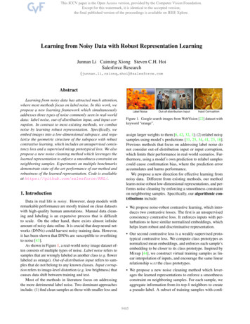
DatasetNoise typeSym 20%CIFAR-10Sym 50% Asym 40%CIFAR-100Sym 20% Sym 50%Cross-Entropy [18]Forward [30]Co-teaching [42]Mixup [44]P-correction [41]MLNT [19]M-correction [1]DivideMix [18]ELR [23] (reproduced)DivideMix (reproduced)82.783.188.292.392.092.093.895.094.7 0.195.1 0.157.959.484.177.688.788.891.993.793.5 0.293.6 0.272.383.188.188.686.391.491.7 0.991.3 0.861.861.464.166.068.167.773.474.875.3 0.275.1 0.237.337.345.346.656.458.065.472.171.3 0.372.1 0.3Ours (classifier)Ours (knn)95.8 0.195.9 0.194.3 0.294.5 0.191.9 0.892.4 0.979.1 0.179.4 0.174.8 0.475.0 0.4Table 1. Comparison with state-of-the-art methods on CIFAR datasets with label noise. Numbers indicate average test accuracy (%) overlast 10 epochs. We report results over 3 independent runs with randomly-generated label noise. Results for previous methods are copiedfrom [1, 18]. We re-run DivideMix and ELR (without model ensemble) using the publicly available code on the same noisy data as ours.Input noiseCEIterative [38]GCE [45]DivideMix [18]Ours (cls.)Ours (knn) CIFAR-100 20k SVHN 20kImage 91.989.891.593.391.493.1 0.393.9 0.291.6 0.2Table 2. Comparison with state-of-the-art methods on CIFAR-10 dataset with label noise (50% symmetric) and input noise (OOD imagesor corrupted images). Numbers indicate average test accuracy (%) over last 10 epochs. We report results over 3 independent runs withrandomly-generated noise. We re-run previous methods using publicly available code with the same data and model as ours.4.2. Experiments on controlled noisy labels withnoisy imagesDataset. We further corrupt a noisy-labeled (50% symmetric) CIFAR-10 dataset by injecting two types of input noise:out-of-distribution (OOD) images and input corruption. ForOOD noise, we follow [38] and add 20k additional imagesfrom either one of the two other datasets: CIFAR-100 andSVHN [28], which enlarges the training set to 70k. A random CIFAR-10 label is assigned to each OOD image. Forinput corruption, we follow [10] and corrupt each image inCIFAR-10 with a noise randomly chosen from the followingfour types: Fog, Snow, Motion blur and Gaussian noise.Examples of both types of input noise are shown in Figure 4.For training, we follow the same implementation details asthe CIFAR-10 experiments described in Section 4.1.Results. Table 2 shows the results. Our method consistentlyoutperforms existing methods by a substantial margin. Weobserve that OOD images from a similar domain (CIFAR100) are more harmful than OOD images from a more different domain (SVHN). This is because noisy images that arecloser to the test data distribution are more likely to distortthe decision boundary in a way that negatively affects testperformance. Nevertheless, performing knn nFogSnowMotion BlurGaussianFigure 4. Examples of input noise injected to CIFAR-10.using the learned embeddings demonstrates high robustnessto input noise.In Figure 5, we show the t-SNE [26] visualization of thelow-dimensional embeddings for all training samples, including in-distribution CIFAR-10 images and out-distributionCIFAR-100 or SVHN images. As training progresses fromepoch 10 to epoch 200, our model learns to separate OODsamples (represented as gray points) from in-distributionsamples (represented as color points). It also learns to cluster CIFAR-10 images according to their true class, despitetheir noisy labels. Therefore, this visualization demonstratesthat the proposed method learns representation that is robustto both label noise and OOD noise.9490

Figure 5. t-SNE visualization of low-dimensional embeddings for CIFAR-10 images (color represents the true class) OOD images (graypoints) from CIFAR-100 or SVHN. The model is trained on noisy CIFAR-10 (50k images with 50% label noise) and 20k OOD images withrandom labels. Our method can effectively learn to (1) cluster CIFAR-10 images according to their true class, despite their noisy labels; (2)separate OOD samples from in-distribution samples, such that their harm is reduced.CIFAR-10 Sym 50% CIFAR-100 20k Image CorruptionCIFAR-100 Sym 50%w/o Lpc mixw/o Lccw/o Lreconw/o mixupw/ standard aug.85.9 (86.1)93.7 (93.8)93.3 (94.0)89.5 (89.9)94.1 (94.3)79.7 (81.5)91.3 (91.5)90.7 (92.9)85.4 (87.0)90.8 (92.9)81.6 (81.7)89.4 (89.5)90.2 (91.0)84.7 (84.9)90.5 (90.7)65.6 (65.9)71.9 (71.8)73.2 (73.9)69.3 (69.7)74.5 (75.0)DivideMixOurs93.694.3 (94.5)89.091.5 (93.1)89.891.4 (91.6)72.174.8 (75.0)Table 3. Effect of the proposed components. We show the accuracy of the classifier (knn) on four benchmarks with different noise. Notethat DivideMix [18] also performs mixup.bottleneck dimensiond 25d 50d 100d 200CIFAR-10 Sym 50%CIFAR-100 Sym 50%93.473.894.374.894.274.493.773.8Table 4. Classifier’s test accuracy (%) with different low-dimensions.4.3. Ablation studythe change of d.Effect of the proposed components. In Table 3, we studythe effect of 5 components from the proposed method including (1) the weakly-supervised mixup prototypical contrastiveloss Lpc mix , (2) the unsupervised consistency contrastiveloss Lcc , (3) the reconstruction loss Lrecon , (4) mixup augmentation, and (5) strong data augmentation with AugMix.We remove each of these components and report the accuracy of the classifier and knn across four benchmarks. Theresult shows that Lpc mix is most crucial to the model’s performance. Lcc has a stronger positive effect with imagecorruption or larger number of classes (CIFAR-100). Ourmethod still achieves competitive performance when eitherthe Lcc or Lrecon is removed. When using standard dataaugmentation (random crop and horizontal flip) instead ofAugMix, our method still achieves state-of-the-art result.Effect of bottleneck dimension. We vary the dimensionality of the bottleneck layer, d, and examine the performancechange in Table 4. Our model is in general not sensitive to4.4. Experiments on real-world noisy dataDataset. Next, we verify our method on two real-word noisydatasets: WebVision [22] and Clothing1M [40]. Webvisioncontains images crawled from the web using the same concepts from ImageNet ILSVRC12 [5]. Following previousworks [3, 18], we perform experiments on the first 50 classesof the Google image subset. Clothing1M consists of imagescollected from online shopping websites where labels weregenerated from surrounding texts. Note that we do not usethe additional clean set for training.Implementation details. For WebVision, we follow previous works [3, 18] and use inception-resnet v2 [33] as theencoder. We train the model using SGD with a weight decayof 0.0001 and a batch size of 64. We train for 40 epochs withan initial learning rate of 0.04. The hyper-parameters areset as d 50, ωcc 1, ωpc 2, ωrecon 1, τ 0.3, α 0.5, η0 0.05, η1 0.8, t0 15. For Clothing1M, we9491

Test datasetWebVisionILSVRC12Accuracy (%)top1top5top1top5Forward [30]Decoupling [27]D2L [25]MentorNet [14]Co-teaching [6]INCV [3]ELR [23]DivideMix 82.482.381.479.984.785.087.889.2Ours (w/o noise cleaning)Ours (classifier)Ours 0.9Table 5. Comparison with state-of-the-art methods trained on WebVision (mini). Numbers denote accuracy (%) on the WebVision validationset and the ImageNet ILSVRC12 validation set. We report results for ELR and DivideMix without model ensemble.MethodCEAccuracy 69.21Forward Joint-Opt ELR MLNT MentorMix69.8472.1672.8773.4774.30SL74.45DivideMix Ours (cls.) Ours (knn)74.4874.9774.84Table 6. Comparison with state-of-the-art methods on Clothing1M dataset. Results for previous methods are directly copied fromcorresponding papers. We report results for ELR and DivideMix without model ensemble.DatasetCIFAR-10Noise typeSym.CIFAR-100Asym.Sym.Noise ratio20%50%80%90%40%20%50

with high-quality human annotations. Manual data clean-ing and labeling is an expensive process that is difficult to scale. On the other hand, there exists almost infinite amount of noisy data online. It is crucial that deep neural net-works (DNNs) could harvest noisy training data. However, it has been shown that DNNs are susceptible to .