Transcription
Donald R. SheehyA First Course onData Structuresin Python
2
Contents1 Overview92 Basic Python2.1 Sequence, Selection, and Iteration . . . . . .2.2 Expressions and Evaluation . . . . . . . . .2.3 Variables, Types, and State . . . . . . . . .2.4 Collections . . . . . . . . . . . . . . . . . .2.4.1 Strings (str) . . . . . . . . . . . . .2.4.2 Lists (list) . . . . . . . . . . . . . .2.4.3 Tuples (tuple) . . . . . . . . . . . .2.4.4 Dictionaries (dict) . . . . . . . . . .2.4.5 Sets (set) . . . . . . . . . . . . . . .2.5 Some common things to do with collections2.6 Iterating over a collection . . . . . . . . . .2.7 Other Forms of Control Flow . . . . . . . .2.8 Modules and Imports . . . . . . . . . . . . .3 Object-Oriented Programming3.1 A simple example . . . . . . . . . . . .3.2 Encapsulation and the Public Interface3.3 Inheritance and is a relationships . . .3.4 Duck Typing . . . . . . . . . . . . . .3.5 Composition and ”has a” relationships4 Testing4.1 Writing Tests . . . . . . . .4.2 Unit Testing with unittest4.3 Test-Driven Development .4.4 What to Test . . . . . . . .3. . . . . .of a Class. . . . . . . . . . . . . . . 345
4CONTENTS4.5Testing and Object-Oriented Design . . . . . . . . . . . . . .465 Running Time Analysis5.1 Timing Programs . . . . . . . . . . . . . . . . . . .5.2 Example: Adding the first k numbers. . . . . . . .5.3 Modeling the Running Time of a Program . . . . .5.3.1 List Operations . . . . . . . . . . . . . . . .5.3.2 Dictionary Operations . . . . . . . . . . . .5.3.3 Set Operations . . . . . . . . . . . . . . . .5.4 Asymptotic Analysis and the Order of Growth . .5.5 Focus on the Worst Case . . . . . . . . . . . . . . .5.6 Big-O . . . . . . . . . . . . . . . . . . . . . . . . .5.7 The most important features of big-O usage . . . .5.8 Practical Use of the Big-O and Common Functions5.9 Bases for Logarithms . . . . . . . . . . . . . . . . .5.10 Practice examples . . . . . . . . . . . . . . . . . .47485355575757585859596060606 Stacks and Queues6.1 Abstract Data Types6.2 The Stack ADT . . .6.3 The Queue ADT . .6.4 Dealing with errors .6363646568.7171727376778283.7 Deques and Linked Lists7.1 The Deque ADT . . . . . . . . . . . . . .7.2 Linked Lists . . . . . . . . . . . . . . . . .7.3 Implementing a Queue with a LinkedList7.4 Storing the length . . . . . . . . . . . . .7.5 Testing Against the ADT . . . . . . . . .7.6 The Main Lessons: . . . . . . . . . . . . .7.7 Design Patterns: The Wrapper Pattern .8 Doubly-Linked Lists858.1 Concatenating Doubly Linked Lists . . . . . . . . . . . . . . . 889 Recursion9.1 Recursion and Induction9.2 Some Basics . . . . . . .9.3 The Function Call Stack9.4 The Fibonacci Sequence.9192929394
CONTENTS9.55Euclid’s Algorithm . . . . . . . . . . . . . . . . . . . . . . . .10 Dynamic Programming10.1 A Greedy Algorithm . . . . . . . . .10.2 A Recursive Algorithm . . . . . . . .10.3 A Memoized Version . . . . . . . . .10.4 A Dynamic Programming Algorithm10.5 Another example . . . . . . . . . . .11 Binary Search11.1 The Ordered List ADT.959999100101102103105. . . . . . . . . . . . . . . . . . . . . 10712 Sorting10912.1 The Quadratic-Time Sorting Algorithms . . . . . . . . . . . . 10912.2 Sorting in Python . . . . . . . . . . . . . . . . . . . . . . . . 11313 Sorting with Divide and Conquer13.1 Mergesort . . . . . . . . . . . . .13.1.1 An Analysis . . . . . . . .13.1.2 Merging Iterators . . . . .13.2 Quicksort . . . . . . . . . . . . .14 Selection14.1 The quickselect algorithm . .14.2 Analysis . . . . . . . . . . . . .14.3 One last time without recursion14.4 Divide-and-Conquer Recap . .14.5 A Note on Derandomization . .15 Mappings and Hash Tables15.1 The Mapping ADT . . . . . . . .15.2 A minimal implementation . . .15.3 The extended Mapping ADT . .15.4 It’s Too Slow! . . . . . . . . . . .15.4.1 How many buckets should15.4.2 Rehashing . . . . . . . . .15.5 Factoring Out A Superclass . . .117. 118. 119. 120. 123.127. 128. 129. 130. 131. 131. . . . . . . . . . . . . . . . .we use?. . . . . . . . .133133134136138140142142
616 Trees16.1 Some more definitions . .16.2 A recursive view of trees .16.3 A Tree ADT . . . . . . .16.4 An implementation . . . .16.5 Tree Traversal . . . . . . .16.6 If you want to get fancy.16.6.1 There’s a catch! . .16.6.2 Layer by Layer . .CONTENTS.17 Binary Search Trees17.1 The Ordered Mapping ADT .17.2 Binary Search Tree Properties17.3 A Minimal implementation .17.3.1 The floor function .17.3.2 Iteration . . . . . . . .17.4 Removal . . . . . . . . . . . . . . . . . . . .and Definitions. . . . . . . . . . . . . . . . . . . . . . . . . . . . . . . . .147. 148. 148. 150. 151. 154. 155. 156. 157.159. 159. 159. 161. 164. 164. 16518 Balanced Binary Search Trees18.1 A BSTMapping implementation . . . . . .18.1.1 Forward Compatibility of Factories18.2 Weight Balanced Trees . . . . . . . . . . .18.3 Height-Balanced Trees (AVL Trees) . . . .18.4 Splay Trees . . . . . . . . . . . . . . . . .16917017117217417519 Priority Queues19.1 The Priority Queue ADT . . . . . . . .19.2 Using a list . . . . . . . . . . . . . . . .19.3 Heaps . . . . . . . . . . . . . . . . . . .19.4 Storing a tree in a list . . . . . . . . . .19.5 Building a Heap from scratch, heapify19.6 Implicit and Changing Priorities . . . .19.7 Iterating over a Priority Queue . . . . .19.8 Heapsort . . . . . . . . . . . . . . . . . .179179180183183185186189189.191. 192. 193. 194. 196.20 Graphs20.1 A Graph ADT . . . . . . . . . . . . . . .20.2 The EdgeSetGraph Implementation . . . .20.3 The AdjacencySetGraph Implementation20.4 Paths and Connectivity . . . . . . . . . .
CONTENTS721 Graph Search21.1 Depth-First Search . . . . . . . . . . . . . . . .21.2 Removing the Recursion . . . . . . . . . . . . .21.3 Breadth-First Search . . . . . . . . . . . . . . .21.4 Weighted Graphs and Shortest Paths . . . . . .21.5 Prim’s Algorithm for Minimum Spanning Trees21.6 An optimization for Priority-First search . . . .201. 202. 204. 205. 206. 209. 21022 (Disjoint) Sets22.1 The Disjoint Sets ADT . .22.2 A Simple Implementation22.3 Path Compression . . . .22.4 Merge by Height . . . . .22.5 Merge By Weight . . . . .22.6 Combining Heuristics . . .22.7 Kruskall’s Algorithm . . .213213214215217218218219
8CONTENTS
Chapter 1OverviewThis book is designed to cover a lot of ground quickly, without taking shortcuts.What does that mean? It means that concepts are motivated andstart with simple examples. The ideas follow the problems. The abstractionsfollow the concrete instances.What does it not mean? The book is not meant to be comprehensive,covering all of data structures, nor is it a complete introduction to all thedetails of Python. Introducing the minimum necessary knowledge to makeinteresting programs and learn useful concepts is not taking shortcuts, it’sjust being directed.There are many books that will teach idiomatic Python programming,and many others that will teach problem solving, data structures, or algorithms. There are many books for learning design patterns, testing, andmany of the other important practices of software engineering. The aim ofthis book is cover many of these topics as part of an integrated course.Towards that aim, the organization is both simple and complex. Thesimple part is that the overall sequencing of the main topics is motivatedby the data structuring problems, as is evident from the chapter titles. Thecomplex part is that many other concepts including problem solving strategies, more advanced Python, object-oriented design principles, and testingmethodologies are introduced bit by bit throughout the text in a logical,incremental way.As a result, the book is not meant to be a reference. It is meant tobe worked through from beginning to end. Many topics dear to my heartwere left out to make it possible to work through the whole book in a singlesemester course.9
10CHAPTER 1. OVERVIEW
Chapter 2Basic PythonThis book is not intended as a first course in programming. It will beassumed that the reader has some experience with programming. Therefore,it will be assumed that certain concepts are already familiar to them, themost basic of which is a mental model for programming that is sometimescalled Sequence, Selection, and Iteration.2.1Sequence, Selection, and IterationA recurring theme in this course is the process of moving from thinkingabout code to writing code. We will try to shape the way we think aboutprograms, the way we write programs, and how we go between the two inboth directions. That is, we want to have facility with both direct manipulation of code as well as high-level description of programs.A nice model for thinking about (imperative) programming is called SequenceSelection-Iteration. It refers to: 1. Sequence: Performing operations oneat a time in a specified order. 2. Selection: Using conditional statementssuch as if to select which operations to execute. 3. Iteration: Repeatingsome operations using loops or recursion.In any given programming language, there are usually several mechanisms for selection and iteration, while sequencing is just the default behavior.In fact, you usually have to have special constructions in a language to dosomething other than performing the given operations in the given order.11
122.2CHAPTER 2. BASIC PYTHONExpressions and EvaluationPython can do simple arithmetic. For example, 2 2 is a simple arithmeticexpression. Expressions get evaluated and produce a value. Some values are numerical like the 2 2 example, but they don’t need to be. Forexample, 5 7 is an expression that evaluates to the boolean value False.Expressions can become more complex by combining many operations andfunctions. For example, 5 * (3 abs(-12) / 3) contains four differentfunctions. Parentheses and the order of operations determine the order thatthe functions are evaluated. Recall that in programming the order of operations is also called operator precedence. In the above example, thefunctions are executed in the following order: abs, /, , *.2.3Variables, Types, and StateImagine you are trying to work out some elaborate math problem withouta computer. It helps to have paper. You write things down, so that you canuse them later. It’s the same in programming. It often happens that youcompute something and want to keep it until later when you will use it. Weoften refer to stored information as state.We store information in variables. In Python, a variable is created byan assignment statement. That is a statement of the form:variable name some valueThe equals sign is doing something (assignment) rather than describingsomething (equality). The right side of is an expression that gets evaluated first. Only later does the assignment happen. If the left side of theassignment is a variable name that already exist, it is overwritten. If itdoesn’t already exist, it is created.The order of evaluation is very important. Having the right side evaluated first means that assignments like x x 1 make sense, because thevalue of x doesn’t change until after x 1 is evaluated. Incidentally, thereis a shorthand for this kind of update: x 1. There are similar notationsfor - , * , and / .An assignment statement is not expression. It doesn’t have a value. Thisturns out to be useful in avoiding a common bug arising from confusing assignment and equality testing (i.e. x y). However, multiple assignmentlike x y 1 does work as you would expect it to, setting both x and yto 1.
2.3. VARIABLES, TYPES, AND STATE13Variables are just names. Every name is associated with some piece ofdata, called an object.The name is a string of characters and it is mapped to an object. The nameof a variable, by itself, is treated as an expression that evaluates to whateverobject it is mapped to. This mapping of strings to objects is often depictedusing boxes to represent the objects and arrows to show the mapping.Every object has a type. The type often determines what you can dowith the variable. The so-called atomic types in Python are integers,floats, and booleans, but any interesting program will contain variables ofmany other types as well. You can inspect the type of a variable using thetype() function. In Python, the word type and class mean the same thing(most of the time).The difference between a variable and the object it represents can getlost in our common speech because the variable is usually acting as the nameof the object. There are some times when it’s useful to be clear about thedifference, in particular when copying objects. You might want to try someexamples of copying objects from one variable to another. Does changingone of them affect the other?x 5y 3.2z Trueprint("x has type", type(x))print("y has type", type(y))print("z has type", type(z))x has type class ’int’ y has type class ’float’ z has type class ’bool’ You should think of an object as having three things: an identity, a type,and a value. Its identity cannot change. It can be used to see if two objectsare actually the same object with the is keyword. For example, considerthe following code.x [1, 2, 3]y xz [1, 2, 3]print(x is y)
14CHAPTER 2. BASIC PYTHONprint(x is z)print(x z)TrueFalseTrueAn object cannot change its identity. In Python, you also cannot changethe type of an object. You can reassign a variable to point to differentobject of a different type, but that’s not the same thing. There are severalfunctions that may seem to be changing the types of objects, but they arereally just creating a new object from the old.x 2print("x ", x)print("float(x) ", float(x))print("x still has type", type(x))print("Overwriting x.")x float(x)print("Now, x has type", type(x))x 2float(x) 2.0x still has type class ’int’ Overwriting x.Now, x has type class ’float’ You can do more elaborate things as well.numstring "3.1415926"y float(numstring)print("y has type", type(y))best number 73x str(best number)print("x has type", type(x))thisworks float("inf")
2.4. COLLECTIONS15print("float(\’inf\’) has type", type(thisworks))infinity plus one float(’inf’) 1y has type class ’float’ x has type class ’str’ float(’inf’) has type class ’float’ This last example introduced a new type, that of a string. A string isa sequence of characters. In Python, there is no special class for a singlecharacter (as in C for example). If you want a single character, you use astring of length one.The value of an object may or may not be changed, depending on thetype of object. If the value can be changed, we say that the object ismutable. If it cannot be changed, we say that the object is immutable.For example, strings are immutable. If you want to change a string, forexample, by converting it to lowercase, then you will be creating a newstring.2.4CollectionsThe next five most important types in Python are strings, lists, tuples,dictionaries, and sets. We call these collections as each can be used forstoring a collection of things. We will see many other examples of collectionsin this course.2.4.1Strings (str)Strings are sequences of characters and can be used to store text of all kinds.Note that you can concatenate strings to create a new string using the plussign. You can also access individual characters using square brackets and anindex. The name of the class for strings is str. You can often turn otherobjects into strings.s "Hello, "t "World."u s tprint(type(u))print(u)print(u[9])
16CHAPTER 2. BASIC PYTHONn str(9876)print(n[2]) class ’str’ Hello, World.r72.4.2Lists (list)Lists are ordered sequences of objects. The objects do not have to be thesame type. They are indicated by square brackets and the elements of thelist are separated by commas. You can append an item to the end of a listL by using the command L.append(newitem). It is possible to index into alist exactly as we did with strings.L [1,2,3,4,5,6]print(type(L)) class ’list’ Here is a common visual representation of the list.L.append(100)You access items by their index. The indices start at 0. Negative indicescount backwards from the end of the list.print("Theprint("Theprint("Theprint("Thefirst item is", L[0])second item is", L[1])last item is", L[-1])second to last item is", L[-2])
2.4. COLLECTIONSTheTheTheThe17first item is 1second item is 2last item is 100second to last item is 6You can also overwrite values in a list using regular assignment statements.L[2] ’skip’L[3] ’a’L[4] ’few’L[-2] 99from ds2.figs import drawlistdrawlist(L, ’list03’)2.4.3Tuples (tuple)Tuples are also ordered sequences of objects, but unlike lists, they areimmutable. You can access the items but you can’t change what items arein the tuple after you create it. For example, trying to append raises anexception.t (1, 2, "skip a few", 99, 100)print(type(t))print(t)print(t[4]) class ’tuple’ (1, 2, ’skip a few’, 99, 100)100Here’s what happens when you try to append.
18CHAPTER 2. BASIC PYTHONt.append(101)Traceback (most recent call last):File "bntsuj6iwl", line 3, in module t.append(101)AttributeError: ’tuple’ object has no attribute ’append’Here’s what happens when you try to assign a value to an item.t[4] 99.5Traceback (most recent call last):File "dar819jypk", line 3, in module t[4] 99.5TypeError: ’tuple’ object does not support item assignmentNote that it would be the same for strings.s ’ooooooooo’s[4] ’x’Traceback (most recent call last):File "6qyosbli42", line 4, in module s[4] ’x’TypeError: ’str’ object does not support item assignment2.4.4Dictionaries (dict)Dictionaries store key-value pairs. That is, every element of a dictionaryhas two parts, a key and a value. If you have the key, you can get thevalue. The name comes from the idea that in a real dictionary (book), aword (the key) allows you to find its definition (the value).The syntax for accessing and assigning values is the same as for lists.
2.4. COLLECTIONS19d dict()d[5] ’five’d[2] ’two’d[’pi’] 3.1415926print(d)print(d[’pi’]){5: ’five’, 2: ’two’, ’pi’: 3.1415926}3.1415926Keys can be different types, but they must be immutable types such asatomic types, tuples, or strings. The reason for this requirement is that wewill determine where to store something using the key. If the key changes,we will look in the wrong place when it’s time to look it up again.Dictionaries are also known as maps, mappings, or hash tables. Wewill go deep into how these are constructed later in the course. A dictionarydoesn’t have a fixed order.If you assign to a key that’s not in the dictionary, it simply creates anew item. If you try to access a key that’s not in the dictionary, you willget a KeyError.D {’a’: ’one’, ’b’: ’two’}D[’c’]Traceback (most recent call last):File "egybsf1d93", line 2, in module D[’c’]KeyError: ’c’2.4.5Sets (set)Sets correspond to our notion of sets in math. They are collections ofobjects without duplicates. We use curly braces to denote them and commasto separate elements. As with dictionaries, a set has no fixed ordering. Wesay that sets and dictionaries are nonsequential collections.Be careful that empty braces indicates an empty dictionary and notan empty set. Here is an example of a newly created set. Some items areadded. Notice that the duplicates have no effect on the value as its printed.
20CHAPTER 2. BASIC PYTHONs )print(s) class ’set’ {1, 2, 3}Be careful, is an empty dictionary. If you want an empty set, you wouldwrite set().2.5Some common things to do with collectionsThere are several operations that can be performed on any of the collectionsclasses (and indeed often on many other types objects).You can find the number of elements in the collection (the length) usinglen.abcde "a string"["my", "second", "favorite", "list"](1, "tuple"){’a’: ’b’, ’b’: 2, ’c’: False}{1,2,3,4,4,4,4,2,2,2,1}print(len(a), len(b), len(c), len(d), len(e))8 4 2 3 4For the sequential types (lists, tuples, and strings), you can slice a subsequence of indices using square brackets and a colon as in the followingexamples. The range of indices is half open in that the slice will start withthe first index and proceed up to but not including the last index. Negativeindices count backwards from the end. Leaving out the first index is thesame as starting at 0. Leaving out the second index will continue the sliceuntil the end of the sequence.
2.6. ITERATING OVER A COLLECTION21Important: slicing a sequence creates a new object. That means a bigslice will do a lot of copying. It’s really easy to write inefficient code thisway.a "a string"b ["my", "second", "favorite", "list"]c (1, )print(c[:2])trinstri[’second’, ’favorite’, ’list’](1, 2)2.6Iterating over a collectionIt is very common to want to loop over a collection. The pythonic way ofdoing iteration is with a for loop.The syntax is shown in the following examples.mylist [1,3,5]mytuple (1, 2, ’skip a few’, 99, 100)myset {’a’, ’b’, ’z’}mystring ’abracadabra’mydict {’a’: 96, ’b’: 97, ’c’: 98}for item in mylist:print(item)for item in mytuple:print(item)for element in myset:print(element)for character in mystring:
22CHAPTER 2. BASIC PYTHONprint(character)for key in mydict:print(key)for key, value in mydict.items():print(key, value)for value in mydict.values():print(value)There is a class called range to represent a sequence of numbers thatbehaves like a collection. It is often used in for loops as follows.for i in range(10):j 10 * i 1print(j, end ’ ’)1 11 21 31 41 51 61 71 81 912.7Other Forms of Control FlowControl flow refers to the commands in a language that affect the orderin which operations are executed. The for loops from the previous sectionis a classic examples of this. The other basic forms of control flow are ifstatements, while loops, try blocks, and function calls. We’ll cover eachbriefly.An if statement in its simplest form evaluates an expression and tries tointerpret it as a boolean. This expression is referred to as a predicate. If thepredicate evaluates to True, then a block of code is executed. Otherwise,the code is not executed. This is the selection of sequence, selection, anditeration. Here is an example.if 3 3 7:print("This should be printed.")if 2 ** 8 ! 256:print("This should not be printed.")This should be printed.
2.7. OTHER FORMS OF CONTROL FLOW23An if statement can also include an else clause. This is a second blockof code that executes if the predicate evaluates to False.if False:print("This is bad.")else:print("This will print.")This will print.A while loop also has a predicate. It is evaluated at the top of a block ofcode. If it evaluates to True, then the block is executed and then it repeats.The repetition continues until the predicate evaluate to False or until thecode reaches a break statement.x 1while x 128:print(x, end ’ ’)x x * 21 2 4 8 16 32 64A try block is the way to catch and recover from errors while a programis running. If you have some code that may cause an error, but you don’twant it to crash your program, you can put the code in a try block. Then,you can catch the error (also known as an exception) and deal with it. Asimple example might be a case where you want to convert some numberto a float. Many types of objects can be converted to float, but manycannot. If we simply try to do the conversion and it works, everything isfine. Otherwise, if there is a ValueError, we can do something else instead.x "not a number"try:f float(x)except ValueError:print("You can’t do that!")You can’t do that!
24CHAPTER 2. BASIC PYTHONA function also changes the control flow. In Python, you define a functionwith the def keyword. This keyword creates an object to store the blockof code. The parameters for the function are listed in parentheses after thefunction name. The return statement causes the control flow to revert backto where the function was called and determines the value of the functioncall.def foo(x, y):return 8 * x yprint(foo(2, 1))print(foo("Na", " batman"))17NaNaNaNaNaNaNaNa batmanNotice that there is no requirement that we specify the types of objectsa function expects for its arguments. This is very convenient, because itmeans that we can use the same function to operate on different types ofobjects (as in the example above). If we define a function twice, even if wechange the parameters, the first will be overwritten by the second. This isexactly the same as assigning to a variable twice. The name of a function isjust a name; it refers to an object (the function). Functions can be treatedlike any other object.def foo(x):return x 2def bar(somefunction):return somefunction(4)print(bar(foo))somevariable fooprint(bar(somevariable))66
2.8. MODULES AND IMPORTS2.825Modules and ImportsAs we start to write more complex programs, it starts to make sense to breakup the code across several files. A single .py file is called a module. Youcan import one module into another using the import keyword. The nameof a module, by default, is the name of the file (without the .py extension).When we import a module, the code in that module is executed. Usually, thisshould be limited to defining some functions and classes, but can technicallyinclude anything. The module also has a namespace in which these functionsand classes are defined.For example, suppose we have the following files.# File: twofunctions.pydef f(x):return 2 * x 3def g(x):return x ** 2 - 1# File: theimporter.pyimport twofunctionsdef f(x):return x - 1print(twofunctions.f(1)) # Will print 5print(f(1))# Will print 0print(twofunctions.g(4)) # Will print 15The import brings the module name into the current namespace. I canthen use it to identify the functions from the module.There is very little magic in an import. In some sense, it’s just telling thecurrent program about the results of another program. Because the import(usually) results in the module being executed, it’s good practice to changethe behavior of a script depending on whether it is being run directly, orbeing run as part of an import. It is possible to check by looking at thename attribute of the module. If you run the module directly (i.e. as ascript), then the name variable is automatically set to main . If themodule is being imported, the name defaults to the module name. Thisis easily seen from the following experiment.
26CHAPTER 2. BASIC PYTHON# File: mymodule.pyprint("The name of this module is", name )The name of this module is main# File: theimporter.pyimport mymoduleprint("Notice that it will print something different when imported?")Here is how we use thebeing run.nameattribute to check how the program isdef somefunction():print("Real important stuff here.")if name ’ main ’:somefunction()Real important stuff here.In the preceding code, the message is printed only when the module isexecuted as a script. It is not printed (i.e. the somefunction function isnot called) if the module is being imported. This is a very common Pythonidiom.One caveat is that modules are only executed the first time they areimported. If, for example, we import the same module twice, it will onlybe executed once. At that point, the namespace exists and can be accessedfor the second one. This also avoids any infinite loops you might try toconstruct by having two modules, each of which imports the other.There are a couple other common variations on the standard importstatement.1. You can import just a particular name or collection of names froma module: from modulename import thethingIwanted. This bringsthe new name thethingIwanted into the current namespace. It doesn’tneed to be preceded by modulename and a dot.
2.8. MODULES AND IMPORTS272. You canimport all the names from the module into the current namespace: from modulename import *. If you do this, every name definedin the module will be accessible in the current namespace. It doesn’tneed to be preceded by modulename and a dot. Although easy to writeand fast for many things, this is generally frowned upon as you oftenwon’t know exactly what names you are importing when you do this.3. You can rename module after importing it: import numpy as np.This allows you to use a different name to refer to the objects of themodule. In this example, I can write np.array instead of numpy.array.The most common reason to do this is to have a shorter name. Theother, more fundamental use is to avoid naming conflicts.
28CHAPTER 2. BASIC PYTHON
Chapter 3Object-Oriente
by the data structuring problems, as is evident from the chapter titles. The complex part is that many other concepts including problem solving strate-gies, more advanced Python, object-oriented design principles, and testing methodologies are introduced bit