Transcription
House Price Prediction Using Machine Learning TechniquesAmmar Alyousfi2018December1
Contents1 Introduction1.1 Goals of the Study . . . . . . . . . . . . . . . . . . . . . . . . . . . . . . . . . . . . . . .1.2 Paper Organization . . . . . . . . . . . . . . . . . . . . . . . . . . . . . . . . . . . . . .4442 Literature Review2.1 Stock Market Prediction Using Bayesian-Regularized Neural Networks . . . . . . .2.2 Stock Market Prediction Using A Machine Learning Model . . . . . . . . . . . . . .2.3 House Price Prediction Using Multilevel Model and Neural Networks . . . . . . .2.4 Composition of Models and Feature Engineering to Win Algorithmic Trading Challenge . . . . . . . . . . . . . . . . . . . . . . . . . . . . . . . . . . . . . . . . . . . . .2.5 Using K-Nearest Neighbours for Stock Price Prediction . . . . . . . . . . . . . . . .4456.883 Data Preparation3.1 Data Description . . . . . . . . . . . .3.2 Reading the Dataset . . . . . . . . . . .3.3 Getting A Feel of the Dataset . . . . .3.4 Data Cleaning . . . . . . . . . . . . . .3.4.1 Dealing with Missing Values .3.5 Outlier Removal . . . . . . . . . . . . .3.6 Deleting Some Unimportant Columns.10101212181825274 Exploratory Data Analysis4.1 Target Variable Distribution . . . . . . . . . . . . . . . . . . . . . . .4.2 Correlation Between Variables . . . . . . . . . . . . . . . . . . . . . .4.2.1 Relatioships Between the Target Variable and Other Varibles4.2.2 Relatioships Between Predictor Variables . . . . . . . . . . .4.3 Feature Engineering . . . . . . . . . . . . . . . . . . . . . . . . . . .4.3.1 Creating New Derived Features . . . . . . . . . . . . . . . .4.3.2 Dealing with Ordinal Variables . . . . . . . . . . . . . . . . .4.3.3 One-Hot Encoding For Categorical Features . . . . . . . . .2727293037404041425 Prediction Type and Modeling Techniques5.0.1 1. Linear Regression . . . . . .5.0.2 2. Nearest Neighbors . . . . . .5.0.3 3. Support Vector Regression .5.0.4 4. Decision Trees . . . . . . . .5.0.5 5. Neural Networks . . . . . .5.0.6 6. Random Forest . . . . . . . .5.0.7 7. Gradient Boosting . . . . . .43434444444445456 Model Building and Evaluation6.1 Feature Scaling . . . . . . . . . . . . . . .6.2 Splitting the Dataset . . . . . . . . . . . .6.3 Modeling Approach . . . . . . . . . . . .6.3.1 Searching for Effective Parameters6.4 Performance Metric . . . . . . . . . . . . .6.5 Modeling . . . . . . . . . . . . . . . . . . .45454646474748.2
6.5.16.5.26.5.36.5.46.5.56.5.66.5.7Linear Regression . . . . . .Nearest Neighbors . . . . .Support Vector Regression .Decision Tree . . . . . . . .Neural Network . . . . . .Random Forest . . . . . . .Gradient Boosting . . . . .485051525354567 Analysis and Comparison7.1 Performance Interpretation . . . . .7.2 Feature Importances . . . . . . . . .7.2.1 XGBoost . . . . . . . . . . . .7.2.2 Random Forest . . . . . . . .7.2.3 Common Important Features.5758626262638 Conclusion659 References653
1IntroductionThousands of houses are sold everyday. There are some questions every buyer asks himself like:What is the actual price that this house deserves? Am I paying a fair price? In this paper, a machinelearning model is proposed to predict a house price based on data related to the house (its size,the year it was built in, etc.). During the development and evaluation of our model, we will showthe code used for each step followed by its output. This will facilitate the reproducibility of ourwork. In this study, Python programming language with a number of Python packages will beused.1.1Goals of the StudyThe main objectives of this study are as follows: To apply data preprocessing and preparation techniques in order to obtain clean data To build machine learning models able to predict house price based on house features To analyze and compare models performance in order to choose the best model1.2Paper OrganizationThis paper is organized as follows: in the next section, section 2, we examine studies related toour work from scientific journals. In section 3, we go through data preparation including datacleaning, outlier removal, and feature engineering. Next in section 4, we discuss the type of ourproblem and the type of machine-learning prediction that should be applied; we also list the prediction techniques that will be used. In section 5, we choose algorithms to implement the techniques in section 4; we build models based on these algorithms; we also train and test each model.In section 6, we analyze and compare the results we got from section 5 and conclude the paper.2Literature ReviewIn this section, we look at five recent studies that are related to our topic and see how models werebuilt and what results were achieved in these studies.2.1Stock Market Prediction Using Bayesian-Regularized Neural NetworksIn a study done by Ticknor (2013), he used Bayesian regularized articial neural network to predictthe future operation of financial market. Specifically, he built a model to predict future stockprices. The input of the model is previous stock statistics in addition to some financial technicaldata. The output of the model is the next-day closing price of the corresponding stocks.The model proposed in the study is built using Bayesian regularized neural network. Theweights of this type of networks are given a probabilistic nature. This allows the network topenalize very complex models (with many hidden layers) in an automatic manner. This in turnwill reduce the overfitting of the model.The model consists of a feedforward neural network which has three layers: an input layer, onehidden layer, and an output layer. The author chose the number of neurons in the hidden layerbased on experimental methods.The input data of the model is normalized to be between -1 and1, and this opertion is reversed for the output so the predicted price appears in the appropriatescale.4
Figure 1: Predicted vs. actual priceThe data that was used in this study was obtained from Goldman Sachs Group (GS), Inc. andMicrosoft Corp. (MSFT) . The data covers 734 trading days (4 January 2010 to 31 December 2012).Each instance of the data consisted of daily statistics: low price, high price, opening price, closeprice, and trading volume. To facilitate the training and testing of the model, this data was splitinto training data and test data with 80% and 20% of the original data, respectively. In additionto the daily-statistics variables in the data, six more variables were created to reflect financialindicators.The performance of the model were evaluated using mean absolute percentage error (MAPE)performance metric. MAPE was calculated using this formula:MAPE ri 1 (abs(yi pi )/yi ) 100r(1)where pi is the predicted stock price on day i, yi is the actual stock price on day i, and r is thenumber of trading days.When applied on the test data, The model achieved a MAPE score of 1.0561 for MSFT part,and 1.3291 for GS part. Figure 1 shows the actual values and predicted values for both GS andMSFT data.2.2Stock Market Prediction Using A Machine Learning ModelIn another study done by Hegazy, Soliman, and Salam (2014), a system was proposed to predictdaily stock market prices. The system combines particle swarm optimization (PSO) and leastsquare support vector machine (LS-SVM), where PSO was used to optimize LV-SVM.The authors claim that in most cases, artificial neural networks (ANNs) are subject to the overfitting problem. They state that support vector machines algorithm (SVM) was developed as analternative that doesn’t suffer from overfitting. They attribute this advantage to SVMs being basedon the solid foundations of VC-theory. They further elaborate that LS-SVM method was reformulation of traditional SVM method that uses a regularized least squares function with equality5
Figure 2: The structure of the model usedconstraints to obtain a linear system that satisfies Karush-Kuhn-Tucker conditions for getting anoptimal solution.The authors describe PSO as a popular evolutionary optimization method that was inspiredby organism social behavior like bird flocking. They used it to find the optimal parameters for LSSVM. These parameters are the cost penalty C, kernel parameter γ, and insensitive loss functionϵ.The model proposed in the study was based on the analysis of historical data and technicalfinancial indicators and using LS-SVM optimized by PSO to predict future daily stock prices. Themodel input was six vectors representing the historical data and the technical financial indicators.The model output was the future price. The model used is represented in Figure 2.Regarding the technical financial indicators, five were derived from the raw data: relativestrength index (RSI), money flow index (MFI), exponential moving average (EMA), stochastic oscillator (SO), and moving average convergence/divergence (MACD). These indicators are knownin the domain of stock market.The model was trained and tested using datasets taken from https://finance.yahoo.com/. Thedatasets were from Jan 2009 to Jan 2012 and include stock data for many companies like Adobeand HP. All datasets were partitioned into a training set with 70% of the data and a test set with30% of the data. Three models were trained and tested: LS-SVM-PSO model, LS-SVM model, andANN model. The results obtained in the study showed that LS-SVM-PSO model had the bestperformance. Figure 3 shows a comparison between the mean square error (MSE) of the threemodels for the stocks of many companies.2.3House Price Prediction Using Multilevel Model and Neural NetworksA different study was done by Feng and Jones (2015) to preduct house prices. Two models werebuilt: a multilevel model (MLM) and an artificial neural network model (ANN). These two modelswere compared to each other and to a hedonic price model (HPM).The multilevel model integrates the micro-level that specifies the relationships between houseswithin a given neighbourhood, and the macro-level equation which specifies the relationshipsbetween neighbouhoods. The hedonic price model is a model that estimates house prices using6
Figure 3: MSE comparisonsome attributes such as the number of bedrooms in the house, the size of the house, etc.The data used in the study contains house prices in Greater Bristol area between 2001 and 2013.Secondary data was obtained from the Land Registry, the Population Census and NeighbourhoodStatistics to be used in order to make the models suitable for national usage. The authors listedmany reasons on why they chose the Greater Bristol area such as its diverse urban and rural blendand its different property types. Each record in the dataset contains data about a house in the area:it contains the address, the unit postcode, property type, the duration (freehold or leasehold), thesale price, the date of the sale, and whether the house was newly-built when it was sold. In total,the dataset contains around 65,000 entries. To enable model training and testing, the dataset wasdivided into a training set that contains data about house sales from 2001 to 2012, and a test setthat contains data about house sales in 2013.The three models (MLM, ANN, and HPM) were tested using three senarios. In the first senario,locational and measured neighbourhood attributes were not included in the data. In the secondsenario, grid references of house location were included in the data. In the third senario, measuredneighbourhood attributes were included in the data. The models were compared in goodness offit where R2 was the metric, predictive accuracy where mean absolute error (MAE) and meanabsolute percentage error (MAPE) were the metrics, and explanatory power. HPM and MLMmodels were fitted using MLwiN software, and ANN were fitted using IBM SPSS software. Figure4 shows the performance of each model regarding fit goodness and predictive accuracy. It showsthat MLM model has better performance in general than other models.7
Figure 4: Model performance comparison2.4Composition of Models and Feature Engineering to Win Algorithmic TradingChallengeA study done by de Abril and Sugiyama (2013) introduced the techniques and ideas used to winAlgorithmic Trading Challenge, a competition held on Kaggle. The goal of the competition wasto develop a model that can predict the short-term response of order-driven markets after a bigliquidity shock. A liquidity shock happens when a trade or a sequence of trades causes an acuteshortage of liquidity (cash for example).The challenge data contains a training dataset and a test dataset. The training dataset hasaround 754,000 records of trade and quote observations for many securities of London StockExchange before and after a liquidity shock. A trade event happens when shares are sold orbought, whereas a quote event happens when the ask price or the best bid changes.A separate model was built for bid and another for ask. Each one of these models consists of Krandom-forest sub-models. The models predict the price at a particular future time.The authors spent much effort on feature engineering. They created more than 150 features.These features belong to four categories: price features, liquidity-book features, spread features(bid/ask spread), and rate features (arrival rate of orders/quotes). They applied a feature selectionalgorithm to obtain the optimal feature set (Fb ) for bid sub-models and the optimal feature set (Fa )of all ask sub-models. The algorithm applied eliminates features in a backward manner in orderto get a feature set with reasonable computing time and resources.Three instances of the final model proposed in the study were trained on three datasets; eachone of them consists of 50,000 samples sampled randomly from the training dataset. Then, thethree models were applied to the test dataset. The predictions of the three models were thenaveraged to obtain the final prediction. The proposed method achieved a RMSE score of 0.77approximately.2.5Using K-Nearest Neighbours for Stock Price PredictionAlkhatib, Najadat, Hmeidi, and Shatnawi (2013) have done a study where they used the k-nearestneighbours (KNN) algorithm to predict stock prices. In this study, they expressed the stock prediction problem as a similarity-based classification, and they represented the historical stock dataas well as test data by vectors.The authors listed the steps of predicting the closing price of stock market using KNN asfollows: The number of neaerest neighbours is chosen8
Figure 5: Prediction performance evaluationFigure 6: AIEI lift graph The distance between the new record and the training data is computed Training data is sorted according to the calculated distance Majority voting is applied to the classes of the k nearest neighbours to determine the predicted value of the new recordThe data used in the study is stock data of five companies listed on the Jordanian stock exchange. The data range is from 4 June 2009 to 24 December 2009. Each of the five companies hasaround 200 records in the data. Each record has three variables: closing price, low price, and highprice. The author stated that the closing price is the most important feature in determining theprediction value of a stock using KNN.After applying KNN algorithm, the authors summarized the prediction performance evaluation using different metrics in a the table shown in Figure 5.The authors used lift charts also to evaluate the performance of their model. Lift chart showsthe improvement obtained by using the model compared to random estimation. As an example,the lift graph for AIEI company is shown in Figure 6. The area between the two lines in the graphis an indicator of the goodness of the model.Figure 7 shows the relationship between the actual price and predicted price for one year forthe same company.9
Figure 7: Relationship between actual and predicted price for AIEI3Data PreparationIn this study, we will use a housing dataset presented by De Cock (2011). This dataset describesthe sales of residential units in Ames, Iowa starting from 2006 until 2010. The dataset contains alarge number of variables that are involved in determining a house price. We obtained a csv copyof the data from et.3.1Data DescriptionThe dataset contains 2930 records (rows) and 82 features (columns).Here, we will provide a brief description of dataset features. Since the number of features islarge (82), we will attach the original data description file to this paper for more information aboutthe dataset (It can be downloaded also from ession-techniques/data). Now, we will mention the feature name with a short description ofits sLotConfigLandSlopeNeighborhoodThe type of the house involved in the saleThe general zoning classification of the saleLinear feet of street connected to the houseLot size in square feetType of road access to the houseType of alley access to the houseGeneral shape of the houseHouse flatnessType of utilities availableLot configurationHouse SlopeLocations within Ames city limits10
FeatureDescriptionCondition1Condition2Proximity to various conditionsProximity to various conditions (if more than one ispresent)House typeHouse styleOverall quality of material and finish of the houseOverall condition of the houseConstruction yearRemodel year (if no remodeling nor addition, same asYearBuilt)Roof typeRoof materialExterior covering on houseExterior covering on house (if more than one material)Type of masonry veneerMasonry veneer area in square feetQuality of the material on the exteriorCondition of the material on the exteriorFoundation typeBasement heightBasement ConditionRefers to walkout or garden level wallsRating of basement finished areaType 1 finished square feetRating of basement finished area (if multiple types)Type 2 finished square feetUnfinished basement area in square feetTotal basement area in square feetHeating typeHeating quality and conditionCentral air conditioningElectrical system typeFirst floor area in square feetSecond floor area in square feetLow quality finished square feet in all floorsAbove-ground living area in square feetBasement full bathroomsBasement half bathroomsFull bathrooms above groundHalf bathrooms above groundBedrooms above groundKitchens above groundKitchen qualityTotal rooms above ground (excluding bathrooms)Home functionalityNumber of FunctionalFireplaces11
ValMoSoldYrSoldSaleTypeSaleConditionFireplace qualityGarage locationYear garage was built inInterior finish of the garageSize of garage (in car capacity)Garage size in square feetGarage qualityGarage conditionHow driveway is pavedWood deck area in square feetOpen porch area in square feetEnclosed porch area in square feetThree season porch area in square feetScreen porch area in square feetPool area in square feetPool qualityFence qualityMiscellaneous featureValue of miscellaneous featureSale monthSale yearSale typeSale condition3.2Reading the DatasetThe first step is reading the dataset from the csv file we downloaded. We will use the read csv()function from Pandas Python package:import pandas as pdimport numpy as npdataset pd.read csv("AmesHousing.csv")3.3Getting A Feel of the DatasetLet’s display the first few rows of the dataset to get a feel of it:# Configuring float numbers formatpd.options.display.float format '{:20.2f}'.formatdataset.head(n 5)12
OrderPIDMS 271050102020202060MS ZoningLot FrontageLot 13830RLRHRLRLRLStreetAlleyLot ShapeLand ContourUtilitiesLot bCornerInsideCornerCornerInsideLand SlopeNeighborhoodCondition 1Condition 2Bldg TypeHouse 1Fam1Fam1Story1Story1Story1Story2StoryOverall QualOverall CondYear BuiltYear 819681998Exterior 1stExterior 2ndMas Vnr TypeBrkFaceVinylSdWd SdngBrkFaceVinylSdPlywoodVinylSdWd SdngBrkFaceVinylSdStoneNoneBrkFaceNoneNoneMas Vnr Area112.000.00108.000.000.0013Roof StyleRoof gCompShgExter QualExter CondTATATAGdTATATATATATA
FoundationBsmt QualBsmt CondBsmt ExposureBsmtFin Type GdNoNoNoNoBLQRecALQALQGLQBsmtFin Type 2BsmtFin SF 2Bsmt Unf SFTotal Bsmt UnfCentral AirElectricalYYYYYSBrkrSBrkrSBrkrSBrkrSBrkrBsmtFin SF 1639.00468.00923.001065.00791.00HeatingHeating QCGasAGasAGasAGasAGasAFaTATAExGd1st Flr SF2nd Flr SFLow Qual Fin SFGr Liv 629Bsmt Full BathBsmt Half BathFull BathHalf BathBedroom AbvGrKitchen 001113233311111Kitchen QualTATAGdExTATotRms 114Fireplace QuGarage TypeGdNaNNaNTATAAttchdAttchdAttchdAttchdAttchd
Garage Yr Blt1960.001961.001958.001968.001997.00Paved DriveGarage FinishGarage CarsGarage 2.00FinUnfUnfFinFinGarage QualGarage CondTATATATATATATATATATAWood Deck SFOpen Porch SFEnclosed Porch3Ssn PorchScreen ol Area00000Pool QCFenceMisc 2NaNNaNYr Sold20102010201020102010Sale TypeSale isc ValMo 0189900Now, let’s get statistical information about the numeric columns in our dataset. We want toknow the mean, the standard deviation, the minimum, the maximum, and the 50th percentile (themedian) for each numeric column in the dataset:dataset.describe(include [np.number], percentiles [.5]) \.transpose().drop("count", axis 1)15
OrderPIDMS SubClassLot FrontageLot AreaOverall QualOverall CondYear BuiltYear Remod/AddMas Vnr AreaBsmtFin SF 1BsmtFin SF 2Bsmt Unf SFTotal Bsmt SF1st Flr SF2nd Flr SFLow Qual Fin SFGr Liv AreaBsmt Full BathBsmt Half BathFull BathHalf BathBedroom AbvGrKitchen AbvGrTotRms AbvGrdFireplacesGarage Yr BltGarage CarsGarage AreaWood Deck SFOpen Porch SFEnclosed Porch3Ssn PorchScreen PorchPool AreaMisc ValMo SoldYr .00800.0017000.0012.002010.00755000.00From the table above, we can see, for example, that the average lot area of the houses in ourdataset is 10,147.92 ft2 with a standard deviation of 7,880.02 ft2. We can see also that the minimumlot area is 1,300 ft2 and the maximum lot area is 215,245 ft2 with a median of 9,436.5 ft2. Similarly,we can get a lot of information about our dataset variables from the table.16
Then, we move to see statistical information about the non-numerical columns in our dataset:dataset.describe(include [np.object]).transpose() \.drop("count", axis 1)MS ZoningStreetAlleyLot ShapeLand ContourUtilitiesLot ConfigLand SlopeNeighborhoodCondition 1Condition 2Bldg TypeHouse StyleRoof StyleRoof MatlExterior 1stExterior 2ndMas Vnr TypeExter QualExter CondFoundationBsmt QualBsmt CondBsmt ExposureBsmtFin Type 1BsmtFin Type 2HeatingHeating QCCentral AirElectricalKitchen QualFunctionalFireplace QuGarage TypeGarage FinishGarage QualGarage CondPaved DrivePool 652652433017
Misc FeatureSale TypeSale Conditionuniquetopfreq5106ShedWDNormal9525362413In the table we got, count represents the number of non-null values in each column, uniquerepresents the number of unique values, top represents the most frequent element, and freq represents the frequency of the most frequent element.3.4Data Cleaning3.4.1 Dealing with Missing ValuesWe should deal with the problem of missing values because some machine learning models don’taccept data with missing values. Firstly, let’s see the number of missing values in our dataset.We want to see the number and the percentage of missing values for each column that actuallycontains missing values.# Getting the number of missing values in each columnnum missing dataset.isna().sum()# Excluding columns that contains 0 missing valuesnum missing num missing[num missing 0]# Getting the percentages of missing valuespercent missing num missing * 100 / dataset.shape[0]# Concatenating the number and perecentage of missing values# into one dataframe and sorting itpd.concat([num missing, percent missing], axis 1,keys ['Missing Values', 'Percentage']).\sort values(by "Missing Values", ascending False)Missing 5.435.362.832.76Pool QCMisc FeatureAlleyFenceFireplace QuLot FrontageGarage CondGarage QualGarage FinishGarage Yr BltGarage TypeBsmt ExposureBsmtFin Type 218
Missing 80.780.070.070.030.030.030.030.030.030.03BsmtFin Type 1Bsmt QualBsmt CondMas Vnr AreaMas Vnr TypeBsmt Half BathBsmt Full BathTotal Bsmt SFBsmt Unf SFGarage CarsGarage AreaBsmtFin SF 2BsmtFin SF 1ElectricalNow we start dealing with these missing values.Pool QC The percentage of missing values in Pool QC column is 99.56% which is very high.We think that a missing value in this column denotes that the corresponding house doesn’t havea pool. To verify this, let’s take a look at the values of Pool Area column:dataset["Pool Area"].value counts()Pool 11111111111We can see that there are 2917 entries in Pool Area column that have a value of 0. This verfiesour hypothesis that each house without a pool has a missing value in Pool QC column and a valueof 0 in Pool Area column. So let’s fill the missing values in Pool QC column with "No Pool":dataset["Pool QC"].fillna("No Pool", inplace True)19
Misc Feature The percentage of missing values in Pool QC column is 96.38% which is veryhigh also. Let’s take a look at the values of Misc Val column:dataset["Misc Val"].value counts()Misc 2211111111111111111111111120
We can see that Misc Val column has 2827 entries with a value of 0. Misc Feature has 2824missing values. Then, as with Pool QC, we can say that each house without a “miscellaneousfeature” has a missing value in Misc Feature column and a value of 0 in Misc Val column. Solet’s fill the missing values in Misc Feature column with "No Feature":dataset['Misc Feature'].fillna('No feature', inplace True)Alley, Fence, and Fireplace Qu According to the dataset documentation, NA in Alley, Fence,and Fireplace Qu columns denotes that the house doesn’t have an alley, fence, or fireplace. Sowe fill in the missing values in these columns with "No Alley", "No Fence", and "No Fireplace"accordingly:dataset[
work. In this study, Python programming language with a number of Python packages will be used. 1.1 Goals of the Study The main objectives of this study are as follows: To apply data preprocessing and preparation techniques in order to obtain clean data To build machine learning m