Transcription
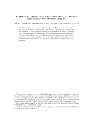
STATISTICAL ESTIMATION: FROM DENOISING TO SPARSEREGRESSION AND HIDDEN CLIQUESERIC W. TRAMEL, SANTHOSH KUMAR, ANDREI GIURGIU, AND ANDREA MONTANARIAbstract. These notes review six lectures given by Prof. Andrea Montanari onthe topic of statistical estimation for linear models. The first two lectures coverthe principles of signal recovery from linear measurements in terms of minimaxrisk. Subsequent lectures demonstrate the application of these principles to several practical problems in science and engineering. Specifically, these topics includedenoising of error-laden signals, recovery of compressively sensed signals, reconstruction of low-rank matrices, and also the discovery of hidden cliques within largenetworks.These are notes from the lecture of Andrea Montanari given at the autumn school “StatisticalPhysics, Optimization, Inference, and Message-Passing Algorithms”, that took place in Les Houches,France from Monday September 30th, 2013, till Friday October 11th, 2013. The school was organizedby Florent Krzakala from UPMC & ENS Paris, Federico Ricci-Tersenghi from La Sapienza Roma,Lenka Zdeborová from CEA Saclay & CNRS, and Riccardo Zecchina from Politecnico Torino.A.M. was partially supported by the NSF grant CCF-1319979 and the grants AFOSR/DARPAFA9550-12-1-0411 and FA9550-13-1-0036.E.W.T. was supported by the ERC under the European Union’s 7th Framework ProgrammeGrant Agreement 307087-SPARCS.1
2E. W. TRAMEL, S. KUMAR, A. GIURGIU, AND A. MONTANARIContentsPreface1. Statistical estimation and linear models1.1. Statistical estimation1.2. Denoising1.3. Least Squares (LS) estimation1.4. Evaluating the estimator2. Nonlinear denoising and sparsity2.1. Minimax risk2.2. Approximation error and the bias-variance tradeoff2.3. Wavelet expansions3. Denoising with thresholding3.1. An equivalent analysis: Estimating a random scalar4. Sparse regression4.1. Motivation4.2. The LASSO4.3. Behavior of the LASSO under Restricted Isometry Property5. Random designs and Approximate Message Passing5.1. Message Passing algorithms5.2. Analysis of AMP and the LASSO6. The hidden clique problem6.1. An iterative thresholding approach6.2. A message passing algorithm6.3. Analysis and optimal choice of ft ( · 5052PrefaceThese lectures provide a gentle introduction to some modern topics in high-dimensionalstatistics, statistical learning and signal processing, for an audience without any previous background in these areas. The point of view we take is to connect the recent advances to basic background in statistics (estimation, regression and the bias-variancetrade-off), and to classical –although non-elementary– developments (sparse estimation and wavelet denoising).The first three sections will cover these basic and classical topics. We will thencover more recent research, and discuss sparse linear regression in Section 4.3.1, andits analysis for random designs in Section 5.2. Finally, in Section 6.3 we discuss anintriguing example of a class of problems whereby sparse and low-rank structureshave to be exploited simultaneously.Needless to say, the selection of topics presented here is very partial. The readerinterested in a deeper understanding can choose from a number of excellent optionsfor further study. Very readable introductions to the fundamentals of statisticalestimation can be found in the books by Wasserman [1, 2]. More advanced references(with a focus on high-dimensional and non-parametric settings) are the monographsby Johnstone [3] and Tsybakov [4]. The recent book by Bühlmann and van de Geer
STATISTICAL ESTIMATION3[5] provides a useful survey of recent research in high-dimensional statistics. For thelast part of these notes, dedicated to most recent research topics, we will providereferences to specific papers.1. Statistical estimation and linear models1.1. Statistical estimation. The general problem of statistical estimation is theone of estimating an unknown object from noisy observations. To be concrete, wecan consider the modely f (θ; noise) ,(1)where y is a set of observations, θ is the unknown object, for instance a vector, a setof parameters, or a function. Finally, f ( · ; noise) is an observation model which linkstogether the observations and the unknown parameters which we wish to estimate.Observations are corrupted by random noise according to this model. The objective isb that is accurate under some metric. The estimationto produce an estimation θb θ(y)of θ from y is commonly aided by some hypothesis about the structure, or behavior,of θ. Several examples are described below.Statistical estimation can be regarded as a subfield of statistics, and lies at thecore of a number of areas of science and engineering, including data mining, signalprocessing, and inverse problems. Each of these disciplines provides some informationon how to model data acquisition, computation, and how best to exploit the hiddenstructure of the model of interest. Numerous techniques and algorithms have beendeveloped over a long period of time, and they often differ in the assumptions andthe objectives that they try to achieve. As an example, a few major distinctions tokeep in mind are the following.Parametric versus non-parametric: In parametric estimation, stringent assumptions are made about the unknown object, hence reducing θ to be determinedby a small set of parameters. In contrast, non-parametric estimation strives tomake minimal modeling assumptions, resulting in θ being an high-dimensionalor infinite-dimensional object (for instance, a function).Bayesian versus frequentist: The Bayesian approach assumes θ to be a randomvariable as well, whose ‘prior’ distribution plays an obviously important role.From a frequentist point of view, θ is instead an arbitrary point in a set ofpossibilities. In these lectures we shall mainly follow the frequentist point ofview, but we stress that the two are in fact closely related.Statistical efficiency versus computational efficiency: Within classical estimation theory, a specific estimator θb is mainly evaluated in terms of its accuracy:bHow close (or far) is θ(y)to θ for typical realizations of the noise? We canbroadly refer to this figure of merit as to ‘statistical efficiency.’Within modern applications, computational efficiency has arisen as a secondcentral concern. Indeed θ is often high-dimensional: it is not uncommon to fitmodels with millions of parameters. The amounts of observations has grownin parallel. It becomes therefore crucial to devise estimators whose complexityscales gently with the dimensions, and with the amount of data.We next discuss informally a few motivating examples.
4E. W. TRAMEL, S. KUMAR, A. GIURGIU, AND A. MONTANARI1.1.1. Example 1: Exploration seismology. Large scale statistical estimation plays akey role in the field of exploration seismology. This technique uses seismic measurements on the earth surface to reconstruct geological structures, composition anddensity field of a geological substrates in [6]. Measurements are acquired, generally, bysending some known seismic wave through the ground, perhaps through a controlledexplosive detonation, and measuring the response at multiple spatially dispersed sensors.Below is a simple dictionary that points at the various elements of the model (1)in this example.Exploration Seismologyyseismographic measurementsθearth density fieldHypothesis smooth density fieldThe function f ( · · · ) in Eq. (1) expresses the outcome of the seismographic measurements, given a certain density field θ and a certain source of seismic waves (leftimplicit since it is known). While this relation is of course complex, and ultimatelydetermined by the physics of wave propagation, it is in principle perfectly known.Because of the desired resolution of the recovered earth density field, this statisticalestimation problem is often ill-posed, as sampling is severely limited by the cost ofgenerating the source signal and the distribution and set-up of the receivers. Resolution can be substantially improved by using some structural insights into the natureof the earth density field. For instance, one can exploit the fact that this is mostlysmooth with the exception of some discontinuity surfaces.Figure 1. A recovered earth density field, from [6].1.1.2. Example 2: Hidden structure in networks. Many modern data sets are relational, i.e. they express pairwise relations within a set of objects. This is the case insocial networks, communication networks, unsupervised learning and so on.In the simplest case, for each pair of nodes in a network, we know whether theyare connected or not. Finding a hidden structure in such a network is a recurringproblem with these datasets. A highly idealized but nevertheless very interestingproblem requires to find a highly connected subgraph in a otherwise random graph.Hidden Network Structureylarge networkθhidden subset of nodesHypothesis hidden network is highly connected
STATISTICAL m Figure 2, it is apparent that the discovery of such networks can be a difficulttask.0.00.20.40.60.81.00.00.40.60.81.0(b) Subgraph hidden.0.00.20.40.60.81.0(a) Subgraph easily visible.0.20.00.20.40.60.81.0(c) Subgraph revealedFigure 2. The same network adjacency matrix, is shown in (a) and(b), but the nodes permuted in (b). In (c), the hidden subgraph isrevealed.1.1.3. Example 3: Collaborative filtering. Recommendation systems are ubiquitousin e-commerce and web services. They aim at personalizing each user’s experiencethrough an analysis of her past behavior, and –crucially– the past behavior of similarusers. The algorithmic and statistical techniques that allow to exploit this information are referred to as ‘collaborative filtering.’ Amazon, Netflix, YouTube all makeintensive use of collaborative filtering technologies.In a idealized model for collaborative filtering, each user of a e-commerce site isassociated to a row of a matrix, and each product to a column. Entry θi,j in thismatrix corresponds to the evaluation that user i gives of product j. A small subsetof the entries is observed because of feedback provided by the users (reviews, ratings,purchasing behavior). In this setting, collaborative filtering aims at estimating thewhole matrix, on the basis of noisy observations of relatively few of its entries.
6E. W. TRAMEL, S. KUMAR, A. GIURGIU, AND A. MONTANARIWhile this task is generally hopeless, it is observed empirically that such datamatrices are often well approximated by low-rank matrices. This corresponds to theintuition that a small number of factors (corresponding to the approximate rank)explain the opinions of many users concerning many items. The problem is thenmodeled as the one of estimating a low-rank matrix from noisy observations of someof its entries.Collaborative Filteringysmall set of entries in a large matrixθunknown entries of matrixHypothesis matrix has a low-rank representationA toy example of this problem is demonstrated in Figures 3-4. It can be observedthat an accurate estimation of the original matrix is possible even when very few ofits coefficients are known.1.2. Denoising. We will begin by considering in greater depth a specific statisticalestimation problem, known as ‘denoising.’ One the one hand, denoising is interesting, since it is a very common signal processing task: In essence, it seeks restorea signal which has been corrupted by some random process, for instance additivewhite-noise. On the other, it will allow us to introduce some basic concepts thatwill play an important role throughout these lectures. Finally, recent research by [7]has unveiled a deep and somewhat surprising connection between denoising and therapidly developing field of compressed sensing.To formally define the problem, we assume that the signal to be estimated is afunction t 7 f (t) Without loss of generality, we will restrict the domain of f (t),f : [0, 1] R. We measure n uniformly-spaced samples over the domain of f ,yi f (i/n) wi ,(2)where i {1, 2, . . . , n} is the sample index, and wi N (0, σ 2 ) is the additive noiseterm. Each of y1 , . . . yn is a sample.For the denoising problem, we desire to calculate the original function from thenoise-corrupted observables yi . How might we go about doing this?1.3. Least Squares (LS) estimation. The Least Squares Method dates backto Gauss and Legendre [8].A natural first idea is to parametrize the function f . For instance we can tentativelyassume that it is a degree p 1 polynomialf (t) pXθj tj 1 .(3)j 1Each monomial is weighted according to coefficient θj for j {1, 2, . . . , p}, and wewill collect these coefficients in a vector θ (θ1 , θ2 , . . . , θp ) Rp . Thus, the problemof recovering f (t) boils down to the recovery of the p coefficients θj from the set ofobservables, yi . We therefore seek to find the set of coefficients which which generatea function that most closely matches the observed samples.
STATISTICAL ESTIMATION7(a) low-rank matrix M(a) low-rank matrix M(b) sampledME(b) sampledMEmatrix(c) output M̂(d) squared 2M M̂matrix(c) output M̂error(d) squared 2M M̂Figure 3. Recovering a2000 2000 rank-8 matrixfrom 0.25% of its values.errorFigure 4. Recovering a2000 2000 rank-8 matrixfrom 1.75% of its values.It is natural to set this up as an optimization problem (here RSS stands for ‘residualsum of squares’)θbLS (y) argmin RSS(θ),(4)θRSS(θ) nXi 1 j 1 !2iyi θj.nj 1pX(5)Fitting a low-degree polynomial to a dataset by least squares is a very commonpractice, and the reader has probably tried this exercise at least once. A moment
8E. W. TRAMEL, S. KUMAR, A. GIURGIU, AND A. MONTANARIFigure 5. Depiction of a discrete-time sampling of the continuoustime function, f (x). Notice that the additive noise term, wi , preventsexact knowledge of f (i/n).reflection reveals that nothing is special about the polynomials used in this procedure.In general, we can consider a set of functions {ϕ1 , ϕ2 , . . . , ϕp }, whereϕj : [0, 1] R.(6)Of course, the quality of our estimate depends on how well the functions {ϕj }capture the behavior of the signal f . Assuming that f can be represented as a linearcombination of these functions, we can rewrite our model asyi pXθ0j ϕj (i/n) wi .(7)j 1Equivalently, if we define ϕ : [0, 1] Rp by lettingPϕ(x) (ϕ1 (x), ϕ2 (x), . . . , ϕp (x)),θ0 (θ0,1 , θ0,2 , . . . , θ0,p ), and denoting by ha, bi mi 1 ai bi the usual scalar productmin R , we haveyi hθ0 , ϕ(i/n)i wi .(8)Before continuing further, it is convenient to pass to matrix notation. Let us definea matrix X (Xij ) Rn p whose entry i, j is given by iXij ϕj,(9)nUsing this notation, and letting y (y1 , y2 , . . . , yn ), w (w1 , w2 , . . . , wn ), our modelreadsy Xθ0 w ,(10)w N (0, σ 2 In ) (here and below In denotes the identity matrix in n dimensions: thesubscript will be dropped if clear from the context).From (10), we see that vector of observations y is approximated as a linear combination of the columns of X, each columns corresponding to one of the functionsϕ1 , ϕ2 , . . . , ϕp , evaluated on the sampling points.
STATISTICAL ESTIMATION9This is a prototype of a very general idea in statistical learning, data mining andsignal processing. Each data point x (or each point in a complicated space, e.g. aspace of images) is represented by a vector in Rp . This vector is constructed byevaluating p functions at x hence yielding the vector (ϕ1 (x), ϕ2 (x), . . . , ϕp (x)). Ofcourse, the choice suitable functions {ϕj } is very important and domain-specific.The functions {ϕj } (or –correspondingly– the columns of the matrix X) have avariety of names. They are known as “covariates” and “predictors” in statistics, as“features” in the context of machine learning and pattern recognition. The set offeatures {ϕj } is sometimes called a “dictionary,” and the matrix X is also referred toas the “design matrix.” Finding an appropriate set of features, i.e. “featurizing”, is aproblem of its own. The observed yi are commonly referred to as the “responses” or“labels” within statistics and machine-learning, respectively. The act of finding thetrue set of coefficients θ0 is known as both “regression” and “supervised learning”.So, how do we calculate the coefficients θ0 from y? Going back to least squaresestimation, we desire to find a set of coefficients, θb which best match our observations.Specifically, in matrix notation (4) readsθbLS argmin L(θ),(11)θ Rpwhere1ky Xθk22 ,2nn1 X(yi hxi , θi)2 , 2n i 1L(θ) (12)with xi Xthe i-th row of X. Here and below kak2 denotes the 2 -norm of vector a:2a2i . The minimizer can be found by noting thatkak2 i1 L(θ) XT (y Xθ),n 1 TLSX y. θb XT X(13)(14)Looking at (14), we note that an important role is played by the sample covariancematrixb 1 XT X.(15)ΣnThis is the matrix of correlations of the predictors {ϕ1 , . . . , ϕp }. The most immediateb needs to be invertible, which is equivalentremark is that, for θbLS to be well defined, Σto require rank (X) p. This of course can only happen if the number of parameterb is invertible butis no larger than the number of observations: n p. Of course, if Σis nearly-singular, then θb will be very unstable and hence a poor estimator. A naturalb is through its condition number κ(Σ),b that isway to quantify the ‘goodness’ of Σb λmax (Σ)/λbbthe ratio of its largest to its smallest eigenvalue: κ(Σ)min (Σ). Fromb 1, whichthis point of view, an optimal design has minimal condition number κ(Σ)corresponds to X to be proportional to an orthogonal matrix. In this case X is calledb (XT X/n) Ipan ‘orthogonal design’ and we shall fix normalizations by assuming Σ
10E. W. TRAMEL, S. KUMAR, A. GIURGIU, AND A. MONTANARIIn functional terms, we see that the LS estimator is calculated according to thecorrelations between y and the predictors,nXb jl 1Σϕj (i/n) ϕl (i/n) ,n i 1 θblLS p Xb 1Σj 1n lj1Xϕj (i/n)yin i 1(16)!.(17)1.4. Evaluating the estimator. Now that we calculated the LS estimator for ourproblem, a natural question arises: is this indeed the best estimator we could use? Inorder to answer this question, we need a way of comparing one estimator to another.This is normally done by considering the risk function associated with the estimator. If the model depends on a set of parameters θ Rp , the risk function is afunction R : Rp R, defined bynob θk2 ,R(θ) E kθ(y)2pnoX E (θ̂j (y) θj )2 .(18)j 1Here expectation is taken with respect to y, distributed according to the model (10)with θ0 θ. Note that the 2 -distance is used to measure the estimation error.Other measures (called ‘loss functions’) could be used as well, but we will focus onthis for the sake of concreteness. We can also calculate risk over the function spaceand not just over the parameter space. This is also known as the ‘prediction error’: n 2 1XbRp (θ) f (i/n) f (i/n)E,n i 1 "#2 pn XX1 EXij θ̂j θj, n i 1 j 1 o1 n E kX θ̂ θ k22 .n(19)In particular, for X an orthogonal design, Rp (θ) c R(θ).Let us apply this definition of risk to the LS estimator, θ̂LS . Returning to the signalsampling model,y Xθ0 w. 1 T θbLS XT XX y, θ0 (XT X) 1 XT w,(20)(21)
STATISTICAL ESTIMATION11which shows that the LS estimator will return the true parameters, θ0 , perturbed bysome amount due to noise. Now, we will calculate the risk functionnoLS2bR(θ) E kθ (y) θ0 k2 ,n 1 T 2 o E k XT XX wk2 ,n 2 T oTT E w X X XX w , 2 T σ 2 Tr X XT XX , 1 σ 2 Tr XT X, b 1σ 2 p Tr Σ ,(22) np1Trp 1bto beΣwhere we add the p term to the final result because we expect thaton the order one, under the assumption of near-orthonormal predictors.Tho further illustrate this point, let us consider the case in which the functions{ϕj } are orthonormal (more precisely, they are an orthonormal set in L2 ([0, 1])).This means thatZ 1ϕi (x)ϕj (x) dx δij .(23)0where δij
Grant Agreement 307087-SPARCS. 1. 2 E. W. TRAMEL, S. KUMAR, A. GIURGIU, AND A. MONTANARI Contents . on how to model data acquisition, computation, and how best to exploit the hidden . Below is a simple dictionary that points