Transcription
Proceedings of the World Congress on Engineering 2011 Vol IWCE 2011, July 6 - 8, 2011, London, U.K.Initial Values in Estimation Procedures for StateSpace Models (SSMs)Raed Alzghool and Yan-Xia LinAbstract—In this paper, we will focus on State Space Models(SSMs), especially the stochastic volatility model, and lookfor a standard approach for assigning initial values in theQuasi-Likelihood (QL) and Asymptotic Quasi-Likelhood (AQL)estimation procedures.Index Terms—State Space Models (SSMs), Quasi-Likelihood(QL), Asymptotic Quasi-Likelhood (AQL), Kalman filter, Nonlinear and/or Non-Gaussian SSMs.I. I NTRODUCTIONTHE class of state space models (SSM) provides aflexible framework for describing a wide range of timeseries in a variety of disciplines. For extensive discussion onSSM and their applications see Harvey [16] and Durbin andKoopman [13]. A state-space model can be written asyt f1 (αt , θ) h1 (yt 1 , θ)ǫt , t 1, 2, · · · , T(1)where y1 , . . . , yT represent the time series of observations;θ is an unknown parameter that needs to be estimated; f1 (.)is a known function of state variable αt and θ; and {ǫt } areuncorrelated disturbances with Et 1 (ǫt ) 0, V art 1 (ǫt ) σǫ2 ; in which Et 1 , and V art 1 denote conditional meanand conditional variance associated with past informationupdated to time t 1 respectively. State variables α1 , . . . , αTare unobserved and satisfy the following modelαt f2 (αt 1 , θ) h2 (αt 1 , θ)ηt , t 1, 2 · · · , T,(2)where f2 (.) is a function of past state variables and θ;{ηt } are uncorrelated disturbances with Et 1 (ηt ) 0,V art 1 (ηt ) ση2 . h1 (.) and h2 (.) are unknown functions.One special application that we will consider in detail isthe Stochastic Volatility Model (SVM), a frequently usedmodel for returns of financial assets. Applications, togetherwith estimation for SVM, can be found in Jacquier, et al[22]; Briedt and Carriquiry [8]; Harvey and Streible [19];Sandmann and Koopman [27]; Pitt and Shepard [25].There are several approaches in the literature for estimating the parameters in SSMs by using the maximumlikelihood method when the probability structure of underlying model is normal or conditional normal. Durbin andKoopman ([14], [13]) obtained accurate approximation ofthe log-likelihood for Non-Gaussian state space models byusing Monte Carlo simulation. The log-likelihood functionis maximised numerically to obtain estimates of unknownparameters. Kuk [23] suggested an alternative class of estimate models based on conjugate latent process and appliedManuscript received March 04, 2011; revised XXXX XX, 2011.R. Alzghool is with the Department of Applied Science, Faculty of PrinceAbdullah Ben Ghazi for Science and Information Technology, Al-Balqa’Applied University, Al-Salt, Jordan e-mail: raedalzghool@bau.edu.jo .Y. Lin is with School of Mathematics and Applied Statistics, University of Wollongong, Wollongong, NSW 2500, Australia e-mail:yanxia@uow.edu.au .ISBN: 978-988-18210-6-5ISSN: 2078-0958 (Print); ISSN: 2078-0966 (Online)it to approximate the likelihood of a time series modelfor count data. To overcome the complex likelihoods ofa time series model with count data, Chan and Ledolter[10] proposed the Monte Carlo EM algorithm that usesa Markov chain sampling technique in the calculation ofthe expectation in the the E-step of the EM algorithm.Davis and Rodriguez-Yam [12] proposed an alternative estimation procedure which is based on an approximationto the likelihood function. Alzghool and Lin [2] proposedquasi-likelihood (QL) approach for estimation of state spacemodels without full knowledge on the probability structureof relevant state-space system. The QL method relaxes thedistributional assumptions and only assumes the knowledgeon the first two conditional moments of yt and αt associatedpast information. This weaker assumption makes the QLmethod widely applicable and become a popular methodof estimation. A comprehensive review on the QL methodis available in Heyde [21]. A limitation of the QL is thatin practice, the conditional second moments of of yt andαt might not available. The AQL approach provides analternative method of parameter estimation when unknownform of heteroscedasticity is presented.The estimation procedure for SSMs consists of two parts.The first part is, given observations {y1 , . . . , yT }, to estimatestate variables αt . The second part is to combine the information of {yt } and {α̂t } to estimate unknown parameter θin the model. The Kalman filter and the smoother methodsare widely used to estimate an unobservable series, statevariables, in SSMs (Anderson and Moore [7], Harvey [17]).In summary, the QL and AQL estimating proceduresdiscussed in Alzghool and Lin ([2],[3], [5]), Alzghool [4],and Alzghool, et al [6]. consist of the following steps:(i) Assign initial values to α0 , θ0 and Σ0 I.(ii) Obtain the QL/AQL estimates α̂t of αt for t 1, 2, . . . , T .(iii) For the AQL estimating procedure, obtain Σ̂t,n byusing the kernel method.(iv) Obtain the QL/AQL estimate θ̂ of θ.(v) Steps (ii), (iii) and (iv) will be alternatively repeateduntil estimates converge.The final estimation results for SSMs might be jointly affected by the initial values α0 and θ0 which initially assignedto the underlying model during the inference procedure.In this paper, following two issues are investigated.(1) How sensitive are the final estimates to the initialvalues assigned to the state variable α0 and θ0 ?(2) If the estimation results are sensitive to the choiceof the initial values, what should initial value of the statevariable α0 be and how is the final estimate of θ determined?This paper is structured as follows. In Section II, thesensitivity of the QL and AQL estimation procedures to theinitial values assigned to state variable α0 is investigatedWCE 2011
Proceedings of the World Congress on Engineering 2011 Vol IWCE 2011, July 6 - 8, 2011, London, U.K.via simulation studies. In Section III, a new suggestion forchoosing the initialisation of the state variable α0 is given.In Section IV, the impact of the starting values of systemparameters θ0 in the estimation results is investigated viasimulation studies. In Section V, a standard procedure toimprove the grid search procedure for obtaining a betterestimation of θ is established. In Section VI applications ofthe QL and AQL methods to real data modelled by SSMsare given. In Section VII, a conclusion is provided.II. E FFECT OF I NITIALISATION OF α0TABLE IQLAND AQL ESTIMATES , BASED ON 1,000 REPLICATIONS . T HE ROOTMEAN SQUARE ERROR OF EACH ESTIMATE IS REPORTED BELOW THATESTIMATE , BASED ON DIFFERENT INITIAL VALUES FOR α0 (T 500).α0true0α̂0 1AQLQLα̂0 2The impact of the initial value of the state variable α0 onthe final inference result is illustrated via simulation studiesin this section. Simulation study based on stochastic volatilitymodel (SVM) is presented below.QLα̂0 3AQLQLA. Stochastic Volatility Models (SVM)Consider the stochastic volatility model,α̂0 4ln(yt2 ) αt ln ξt 2 , t 1, 2, · · · , T,(3)αt γ φαt 1 ηt , t 1, 2, · · · , T,(4)AQLQLwhere both ξt and ηt are i.i.d. r.v.’s; ηt has mean 0 andvariance ση2 .In order to show how the initial value α0 effects the finalestimation in the SVM when the QL and AQL approaches areapplied, we carried out a simulation study on SVM Modeldefined by (3) and (4). The simulation was conducted asfollows. First, 1,000 independent samples of size 500 aregenerated from (3) and (4) based on a true parameter θ (γ, φ), where ηt N (0, ση2 ), ξt N (0, 1), and the initialvalue for α0 in the true model is α0 0. Once {yt } and{αt } are generated, pretend that {αt } is unobserved and γ,and φ are unknown. Then apply the QL and AQL estimationprocedures to {yt } only to obtain the estimate of αt , γ, andφ. Different parameter settings for (γ, φ, ση2 ) are consideredin the simulation. The mean and root mean squared errors forγ̂ and φ̂ based on 1,000 independent samples are calculated.Let α̂0 be the initial state used in the inference procedure.In Table I, different values of α̂0 , mean and root meansquared errors for γ̂, and φ̂ given by the QL and AQLmethods are reported.We can see from Table I that the RMSE of QL and AQLestimates are increased when α̂0 is chosen farther from thetrue value α0 . Since the increase in the RMSE for QL isless than for AQL, this indicates that the QL approach isless sensitive to the initial value of state variable than theAQL approach.III. D ETERMINATION OF α̂0Consider the univariate time series yt satisfyingyt αt ǫt , t 1, 2, · · · , T(5)αt αt 1 ηt , t 1, 2, · · · , T(6)where ǫt N (0, σǫ2 ), ηt N (0, ση2 ), and α0 N (a0 , P0 ).{ǫt } and {ηt } are two independent Gaussian white noiseseries. The initial value α0 is independent of {ǫt } and {ηt }for t 0. In literature, αt is referred to as the trend of theISBN: 978-988-18210-6-5ISSN: 2078-0958 (Print); ISSN: 2078-0966 (Online)AQLση 0.675γ φ-0.8210.90ση 0.260γ φ-0.368ση 0.061γ φ0.95-0.1410.98-0.873 0.9150.138 0.020-0.843 0.9310.141 0.033-0.411 0.9240.234 0.047-0.431 0.9270.098 0.025-0.349 0.9540.255 0.036-0.228 0.9640.091 0.017-0.860 0.9160.136 0.022-0.893 0.9270.159 0.029-0.328 0.9340.210 0.046-0.482 0.9200.134 0.032-0.230 0.9700.157 0.021-0.250 0.9700.120 0.022-0.817 0.9160.169 0.032-0.935 0.9230.179 0.026-0.255 0.9330.307 0.076-0.527 0.9130.175 0.039-0.157 0.9820.112 0.021-0.286 0.9540.149 0.027-0.770 0.9120.240 0.045-0.965 0.9210.198 0.024-0.144 0.9210.442 0.084-0.574 0.9050.219 0.049-0.089 0.9820.237 0.042-0.318 0.9490.178 0.032series, which is not directly observable, and yt is observable.The model is called a local level model in Durbin andKoopman ([13], Chapter 2), which is a simple case of thestructural time series model of Harvey [17].When nothing is known about the initial value α0 , the initialisation of α0 is usually given by a diffuse prior approachthat fixes a0 at an arbitrary value and let P0 (Zivot etal. [30], Durbin and Koopman [13], Harvey [16]). However,some researchers consider that the diffuse approach is notrealistic because they regard that the assumption of infinitevariance is unnatural, given that all observed time series havefinite values. From this point of view an alternative approachis suggested, which assumes that α0 is an unknown constantand needs to be estimated from the data. In Harvey [18],it is suggested that the initial value of α0 can be taken asy1 . This is the same value as that obtained by assumingthat α0 is diffuse. More details about the intitialisation ofthe Kalman filter under the normality assumption for SSMare provided in Durbin and Koopman ([13], Chapter 5 andreferences therein). Several other suggestions on initialisationfor the state variable in SSM under normality assumptionare given in a recent survey by Casals and Sotoca [9]. Theyderived an exact expression for the conditional mean andvariance of the initial state of SSM.In this paper, we follow the QL method to derive a simplemethod for determining α̂0 without assigning any probabilitydistribution to α0 .Consider the following state-space model:yt f (αt , θ) ǫt , t 1, 2, · · · , T,(7)αt g(αt 1 , θ) ηt , t 1, 2 · · · , T.(8)For t 1, we havey1 f (α1 , θ) ǫ1 ,(9)α1 g(α0 , θ) η1 .(10)WCE 2011
Proceedings of the World Congress on Engineering 2011 Vol IWCE 2011, July 6 - 8, 2011, London, U.K.In models (9), and (10), α1 , α0 , ǫ1 , and η1 are unobserved.Assume θ is known or determined by empirical knowledge.The rule used to determine α̂0 should meet the conditionthat given observation y1 , α̂0 is able to ensure that f (α̂1 , θ)is an optimal estimation of E(y1 ).From (9), considerǫ1 y1 f1 (α1 , θ)TABLE IIQLAND AQL ESTIMATES BASED ON 1,000 REPLICATION . T HE ROOTMEAN SQUARE ERROR OF EACH ESTIMATE IS REPORTED BELOW THATESTIMATE . α̂ 0 IS DIFFERENT FROM SAMPLE TO SAMPLE . (T 500).α0true0α0 0AQLQLLet α1 be an unknown parameter and consider estimatingfunction spaceα0 α̂ 0(1)GTAQL {a1 (y1 f1 (α1 , θ)) a1 R}.QLA standardised optimal estimating function inG (1) (α1 ) E((1)GTis f)[V ar(ǫ1 )] 1 (y1 f (α1 , θ)). α1ση 0.061γ φ-0.821-0.368-0.1410.900.950.98-0.878 0.920.136 0.019-0.788 0.940.140 0.037-0.499 0.910.229 0.049-0.391 0.940.071 0.019-0.437 0.940.354 0.052-0.198 0.970.063 0.013-0.857 0.920.163 0.024-0.830 0.930.142 0.034-0.499 0.910.243 0.051-0.378 0.940.082 .019-0.440 0.940.402 0.060-0.194 0.970.071 .014Consider stochastic volatility process defined by (3) and(4), i.e.ln(yt2 ) αt ln ξt 2 , t 1, 2, · · · , T.(11)αt γ φαt 1 ηt , t 1, 2, · · · , T,Using (10), considerη1 α1 g(α0 , θ).Let α0 be an unknown parameter and consider estimatingfunction space(0)(0)A standardised optimal estimating function in GTǫ1is g)[V ar(η1 )] 1 (α1 f (α0 , θ)). α0(12)Therefore, we make the following suggestion for determiningthe initial state α̂0 in inference process.Suggestion: For a SSMαt g(αt 1 , θ) ηt , t 1, 2 · · · , T. f gIf E( α) 6 0, E( α) 6 0, f 1 and g 1 exist, the optimal10decision on α̂0 isα̂0 g(f 1(y1 )).(13)For convenience, denote this α̂0 as α̂0 .As an example for (5) and (6), the optimal value for α̂0is y1 , which is the same as the one given under diffuseconditions.In the following, we apply the Suggestion to stochasticvolatility model, and use simulation to investigate whetherthe Suggestion is practicable or not.ISBN: 978-988-18210-6-5ISSN: 2078-0958 (Print); ISSN: 2078-0966 (Online)ln(y12 ) α1 E(ln ξ1 2 )ln(y12 ) f (α1 , θ),η1 α1 (γ φα0 )α1 g(α0 , θ),where θ (γ, φ)′ , f (α1 , θ) α1 E(ln ξ1 2 ), andg(α0 , θ) γ φα0 . f gSince E( α) 1 6 0, E( α) φ 6 0, and f 1 , g 110exist, therefore,α̂0 g 1 (f 1 (y1 )) yt f (αt , θ) ǫt , t 1, 2, · · · , T 1 and gIf E( α) 6 0, and g 1 exists, the optimal estimator of α00will given by G (0) (α0 ) 0, that is,α̂0 g 1 (α1 , θ).where both ξt and ηt are i.i.d. r.v.’s; ηt has mean 0 andvariance ση2 , φ 6 0.Letǫ1 ln ξ1 2 E(ln ξ1 2 ).Using (3) and (4), it follows thatGT {a0 (α1 g(α0 , θ)) a0 R}.G (0) (α0 ) E(ση 0.260γ φA. Stochastic Volatility Model fIf E( α) 6 0, and f 1 exists, the optimal estimator of1α1 will be given by G (1) (α1 ) 0, that is,α̂1 f 1 (y1 , θ).ση 0.675γ φln(y12 ) E(ln ξ1 2 ) γ.φ(14)If ξt has standard normal distribution, then E(ln ξt2 ) 1.2704 and V ar(ln ξt2 ) π 2 /2 (see Abramowitz andStegun [1], p. 943). Then, substituting in (14)α̂0 g 1 (f 1 (y1 )) ln(y12 ) 1.2704 γ.φ(15)To show how the optimal initial value α̂0 effects the finalestimation when the QL and AQL approaches are applied,we carried out a simulation study on SVM model defined by(3) and (4). We camper the estimation of (, φ) given by thetrue α0 and α̂0 . Results are presented by Table II.Table II shows that, compared to results in Table I, theestimation given by α̂0 are close related to those given bythe true α0 0.WCE 2011
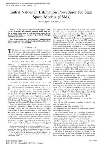
Proceedings of the World Congress on Engineering 2011 Vol IWCE 2011, July 6 - 8, 2011, London, U.K.Fig. 1. Histogram of QL estimation of γ in SVM, based on 2,000 differentstarting values.Fig. 2. Histogram of QL estimation of φ in SVM, based on 2,000 differentstarting values.IV. T HE S TARTING VALUES FOR S YSTEM PARAMETER θ0In this section, we consider the starting value for systemparameters θ0 . As described in literature, the outputs of nonlinear inference procedures rely strongly on the appropriatevalue of the initial parameter θ0 . It is usually suggestedthat θ0 should be chosen from a close neighbourhood ofits true value (Zivot et al. [30]). Since the true value ofθ0 is unknown, it is an issue how to identify the closeneighbourhood of θ0 .The impact of the starting values of system parameters θ0is illustrated via simulation studies below.A. Stochastic Volatility ModelsConsider SVM as given in (3) and (4) where ηt N (0, 0.6752 ), ξt N (0, 1), and the initial value for α0 inthe true model is given by α0 0. In this example, the statespace model is involved with the parameter θ (γ, φ). Letθ ( 0.368, 0.95), a sequence of observations y1 , · · · , y1000from the state space model were generated. Then we pretend θ is unknown. Consider a two-dimensional range (0.868,0.132; 0.80,0.99) for θ (γ, φ), which covers the trueparameter (-0.368,0.95). Then we apply a two-dimensionalgrid search to (-0.868,0.132; 0.80,0.99) with increasment of0.01. For each starting value of θ from the grid area, we applythe QL and AQL estimating procedures to the realisationy1 , · · · , y1000 and obtain the QL and AQL estimation of θwhere α̂0 α0 are used. In Figure 1 - 4, we show thehistograms of QL and AQL estimation of γ and φ based on2000 different starting values.Like others estimation procedures described in literature,the QL and AQL estimations of θ rely strongly on the valueof the initial parameter θ0 .We note an interesting phenomenon in the histogramsillustrated in Figures 1 - 4. The true value of a parameter isnot always allocated in the low frequency area. Obviously,the size of the low frequency area relies on the natureof the true model. This suggests that, although it is notappropriate to quantitatively identify an optimal estimationon system parameters utilising the information providedby a histogram diagram indirectly through the grid searchapproach, it is possible to narrow down and obtain a potentialISBN: 978-988-18210-6-5ISSN: 2078-0958 (Print); ISSN: 2078-0966 (Online)Fig. 3. Histogram of AQL estimation of γ in SVM, based on 2,000 differentstarting values.Fig. 4. Histogram of AQL estimations of φ in SVM, based on 2,000different starting values.range covering the true value of parameters in underlyingmodel by using the information provided by the histogramdiagrams.WCE 2011
Proceedings of the World Congress on Engineering 2011 Vol IWCE 2011, July 6 - 8, 2011, London, U.K.V. D ETERMINATION OF THE E STIMATION OF THES YSTEM PARAMETER θIn their survey article, Zivot et al. [30] suggested choosinga starting value θ0 close to the true value of θ. The estimationof θ using a Monte Carlo approximation for count datagiven by Kuk [23] is only good when the initial value ofθ is assigned around the true value of θ. Other approachesto decide θ0 are also suggested in literatuer. For example,Durbin and Koopman [14] numerically maximised the approximate likelihood for non-Gaussian SSMs to obtain thestarting value for θ0 ; Sandmann and Koopman [27] used atwo-dimensional grid search procedure which searches foran appropriate starting value for θ0 across the surface of aGaussian log-likelihood function; Geweke and Tanizaki [15]and Tanizaki and Mariano ([28], [29]) used a simple gridsearch for θ0 where the expected log-likelihood function ismaximised.The ML method is a popular method for estimating theparameters of SSMs. The ML method works if the probability structure of the underlying state space system is known.In practice, it is not realistic to assume that the system’sprobability structure is known. Then, the maximum likelihood method becomes impracticable. Therefore, searching θ0based on maximising the log-likelihood function cannot beapplied. Without knowledge of the log-likelihood, a distribution free procedure can be considered. It is implemented by agrid search over a feasible region of the parameter space, andthe parameter estimation will be the one giving the minimumresidual sum of squares (RSS)( see Coakley et al. [11] andNaik-nimbalkar and Rajarshi [24]).In this paper, we adapt grid search procedure but withsome improvements. It is sensible to obtain the estimateof θ by utilising a the grid search, and the residual sumof squares. However, if the grid search area is relativelylarge, the smallest sum of residuals might not lead to thebest estimation of θ. One example can be fond from thesimulation study discussed below. To improve the outcomesof the grid search procedure and sum of residuals, we needto reduce the area of the grid search into a reasonable si
R. Alzghool is with the Department of Applied Science, Faculty of Prince Abdullah Ben Ghazi for Science and Information Technology, Al-Balqa’ Applied University, Al-Salt, Jordan e-mail: raedalzghool@bau.edu.jo . Y. Lin is with School of Mathematics and Applied Statistics, Uni-versi