WIXLIB

APRIL 2010Mebane T. FaberPortfolio ManagerCAMBRIA INVESTMENT MANAGEMENT, INC.Relative Strength Strategies for InvestingFirst DraftApril 2010ABSTRACTThe purpose of this paper is to present simple quantitative methods that improve risk-adjusted returns forinvesting in US equity sector and global asset class portfolios. A relative strength model is tested on theFrench-Fama US equity sector data back to the 1920s that results in increased absolute returns with equity-likerisk. The relative strength portfolios outperform the buy and hold benchmark in approximately 70% of all yearsand returns are persistent across time. The addition of a trendfollowing parameter to dynamically hedge theportfolio decreases both volatility and drawdown. The relative strength model is then tested across a portfolioof global asset classes with supporting ainvestments.com/www.mebanefaber.com2321 ROSECRANS AVE., SUITE 4210EL SEGUNDO, CA 90245(310) 606-5555Electronic copy available at: http://ssrn.com/abstract 1585517

MOMENTUMMomentum based strategies, in which we group both trendfollowing and relative strength techniques, have beenapplied as investment strategies for over a century. Momentum has been one of the most widely discussed andresearched investment strategies (some academics would prefer the term “anomaly”).This paper is not an attempt to summarize the momentum literature. There are numerous sources that havedone a fine job on that front already including:On the Nature and Origins of Trendfollowing – Stig OstgaardThe Case for Momentum Investing – AQR WebsiteBringing Real World Testing to Relative Strength – John LewisGlobal Investment Returns Yearbook – Dimson, Marsh, StauntonAppendix in Smarter Investing in Any Economy – Michael CarrTrendfollowing – Michael CovelThe Capitalism Distribution – BlackStar FundsAnnotated Bibliography of Selected Momentum Research Papers – AQR WebsiteNor is this paper an attempt to publish an original and unique method for momentum investing. Similarsystems and techniques to those that follow in this paper have been utilized for decades. Rather, our intent is todescribe some simple methods that an everyday investor can use to implement momentum models in trading.The focus is on the practitioner with real world applicability.www.cambriainvestments.comElectronic copy available at: http://ssrn.com/abstract 15855172

DATAThis research report utilizes the French-Fama CRSP Data Library since it has the longest history and is widelyrelied upon and accepted in the research community. Specifically, we are using the 10 Industry Portfolios withmonthly returns from July 1926 through December 2009, encompassing over eight decades of US equity sectorreturns. Our study begins in 1928 since a year is needed for a ranking period. We utilize the value weightedgroupings rather than the less realistic equal weighted portfolios, and the sectors are described below:Consumer Non-Durables -- Food, Tobacco, Textiles, Apparel, Leather, ToysConsumer Durables -- Cars, TV's, Furniture, Household AppliancesManufacturing -- Machinery, Trucks, Planes, Chemicals, Office Furniture, Paper, Commercial PrintingEnergy -- Oil, Gas, and Coal Extraction and ProductsTechnology -- Computers, Software, and Electronic EquipmentTelecommunications -- Telephone and Television TransmissionShops -- Wholesale, Retail, and Some Services (Laundries, Repair Shops)Health -- Healthcare, Medical Equipment, and DrugsUtilitiesOther -- Mines, Construction, Transportation, Hotels, Business Services, Entertainment, FinanceData for the global asset classes are obtained from Global Financial Data and described in the Appendix.www.cambriainvestments.com3

SECTOR RETURNSIn the United States the 20th Century experienced strong returns for an equity investor.Exhibit 1 – US Equity Sector Total Returns, 1928-2009www.cambriainvestments.com4

Exhibit 2 – US Equity Sector Total Returns, 1928-2009For comparison we have included a portfolio that is equal weighted among the ten sectors, rebalanced monthly,as well as the S&P 500.Exhibit 3 – US Equity Total Returns, 1928-2009www.cambriainvestments.com5

Investors received strong returns for equities, but they were not without risk. Volatility and massive drawdownswere commonplace. Below we will examine a method for momentum investing, specifically relative strength.Below are the buy and sell rules for the system.RANKINGEach month the ten sectors are ranked on trailing total return including dividends. We use varying periods ofmeasurement ranging from one to twelve months, as well as a combination of multiple months.For example: If we are examining relative strength at the one month interval on December 31st 2009, we wouldsimply sort the ten sectors by their prior month (December 2009) total returns including dividends. For thethree month period, we would sort the ten sectors by their three month (October 2009-December 2009) totalreturns including dividends.BUY RULEThe system invests in the top X sectors. For Top 1, the system is 100% invested in the top ranked sector. ForTop 2, the system is 50% invested in each of the top two sectors. For Top 3, the system is 33% invested in eachof the top three sectors.SELL RULESince the system is a simple ranking, the top X sectors are held and if a sector falls out of the top X sectors it issold at the monthly rebalance and replaced with the sector in the top X.www.cambriainvestments.com6

1. All entry and exit prices are on the day of the signal at the close. The model is only updated once a monthon the last day of the month. Price fluctuations during the rest of the month are ignored.2. All data series are total return series including dividends, updated monthly.3. Taxes, commissions, and slippage are excluded (see the Real World Implementation section later in thepaper).Below are summaries of the various ranking periods and returns for the portfolios. The 1, 3, 6, 9, and 12 monthcombination simply takes an average of the five rolling returns for each sector every month to sort the 10sectors.www.cambriainvestments.com7

Exhibit 4.1 – 1 Month Relative Strength Portfolios, 1928-2009Exhibit 4.2 – 3 Month Relative Strength Portfolios, 1928-2009Exhibit 4.3 – 6 Month Relative Strength Portfolios, 1928-2009Exhibit 4.4 – 9 Month Relative Strength Portfolios, 1928-2009Exhibit 4.5 – 12 Month Relative Strength Portfolios, 1928-2009www.cambriainvestments.com8

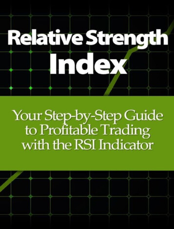
Exhibit 4.6 – Combination 1, 3, 6, 9 and 12 Month Relative Strength Portfolios, 1928-2009From the above tables it is apparent that the relative strength method works on all of the measurement periodsfrom one month to twelve months, as well as a combination of the 1, 3, 6, 9, and 12 month time periods. Moreinteresting is that the system outperforms buy and hold in roughly 70% of all years. Below is an equity curvefor the combination measurement system. A rough estimate of 300-600 basis points of outperformance per yearis reasonable.www.cambriainvestments.com9

Exhibit 5 – Relative Strength Portfolios, 1928-2009www.cambriainvestments.com10

Exhibit 6 shows the outperformance by decade for the relative strength strategy on a yearly compounded basis.For example, the Top 1 beat the buy and hold portfolio by 2.68% a year in the 1930s.Exhibit 6 – Relative Strength Portfolios, CAGR Outperformance by Decade 1928-2009SOLUTIONS TO THE DRAWBACKS OF RELATIVE STRENGTH SYSTEMSThe biggest drawback of a relative strength system is that the portfolio is long-only and fully invested, thusleaving the portfolio exposed to the risks of that particular asset beta. In this case the investor is exposedprimarily to US stock risk. This detail can be seen in the volatility and drawdowns of all of the portfolios.There are two possible solutions to control for the losses and drawdowns while using a relative strength rotationsystem: (1) hedging and, (2) adding non-correlated asset classes.Solution 1: Hedging (either moving to cash or hedging with shorts). Hedging can be done on a sector basisor on a portfolio wide asset class basis. An investor could utilize a static hedge that always hedges a percentageof the portfolio, or possibly the entire portfolio (market neutral). This hedging technique has the drawback ofhedging the portfolio when the market is appreciating, but also protects against all declines and shocks. Anwww.cambriainvestments.com11

investor could also use options to gain short exposure (essentially acting as insurance), with a cost, to theportfolio.Another hedging option is a dynamic hedging technique that attempts to hedge when conditions are morefavorable to market declines. Consistent with research we published in "A Quantitative Approach to TacticalAsset Allocation", using a long term moving average to hedge a portfolio results in a reduction in volatility anddrawdown versus buy and hold. This approach can be seen in this research piece we published on tradingFidelity Sector Funds, “Combining Rotation and Timing Systems”. Below we examine the combination of the1, 3, 6, 9, and 12 month sector rotation portfolios when they are dynamically hedged. The portfolios moveentirely to 100% cash (T-Bills) when the S&P 500 is below its 10 month Simple Moving Average (SMA).(Note: This system could also be run individually on the sectors with similar results.)Exhibit 7 – Dynamically Hedged Combination 1, 3, 6, 9 and 12 MonthRelative Strength Portfolios, 1928-2009By adding the dynamic hedge, most portfolios preserve their returns (although the Top 1 takes a 150 basis pointhit), but have the added benefit of reduced volatility and drawdowns. While an approximate 40-50% drawdownis still large, it is more tolerable than a 70-80% drawdown.www.cambriainvestments.com12

Solution 2: Addition of non-correlated asset classes. The second possible solution to the drawback of singleasset class exposure inherent in the US sector rotation strategy is to add non-correlated global asset classes tothe portfolio. Just as we have demonstrated above that a momentum strategy works in US equity sectors, so toodoes momentum work across global asset classes. We detailed this method in our book The Ivy Portfolio with aglobal rotation system that adds foreign stocks, bonds, REITs, and commodities to the portfolio. Other assetclasses and spreads could be included to further diversify the portfolio, but examining this simple five assetclass portfolio is instructive.Below are the returns of the five asset classes we examine in this paper since 1973. The buy and holdbenchmark is an equal-weighted portfolio of the five asset classes, rebalanced monthly.Exhibit 8 – Global Asset Class Total Returns, 1973-2009www.cambriainvestments.com13

Exhibit 9 – Global Asset Class Total Returns, 1973-2009Below are summaries of the various ranking periods and returns for the portfolios.www.cambriainvestments.com14

Exhibit 10.1 – 1 Month Relative Strength Portfolios, 1973-2009Exhibit 10.2 – 3 Month Relative Strength Portfolios, 1973-2009Exhibit 10.3 – 6 Month Relative Strength Portfolios, 1973-2009Exhibit 10.4 – 9 Month Relative Strength Portfolios, 1973-2009www.cambriainvestments.com15

Exhibit 10.5 – 12 Month Relative Strength Portfolios, 1973-2009Exhibit 10.6 – Combination 1, 3, 6, 9, and 12 Month Relative Strength Portfolios, 1973-2009From the above tables it is apparent that the relative strength method works on all of the measurement periodsfrom one month to twelve months, as well as a combination of time periods. More interesting is that the systemoutperforms buy and hold in roughly 70% of all years. A rough estimate of 300-600 basis points ofoutperformance per year is reasonable. Below is an equity curve:www.cambriainvestments.com16