Transcription
Introduction to PODS PassengerChoice ModelDr. Peter P. Belobaba16.75J/1.234J Airline ManagementFebruary 27, 20061
Overview of PODS ArchitectureMultiple iterations (samples) of pre-departurebooking process and departure day:4 Stationary process (no trends)4 Initial input values for demands, then gradual replacementwith direct observations4 “Burn” first n observations in calculating final scoresPre-departure process broken into time frames:4 RM system intervention at start of each time frame4 Bookings arrive randomly during time frame4 Historical data base updated at end of time frame2
PODS Simulation: Basic UPDATEHISTORICALBOOKINGDATA BASE3HISTORICALBOOKINGS
PODS Demand InputsTotal daily demand for an O-D market, by passengertype (business vs. leisure).Booking curves by passenger type over 16 bookingperiods before departure.Correlation parameters between passenger typesand across booking periods.4
Booking Arrival Curves by PAX Type100%90%80%Percent 423531282421Days Out51714107531
Business vs. Leisure PassengersTwo passenger types defined by:4 Time of day demand and schedule tolerance4 Maximum out-of-pocket fare willingness to pay4 “Attributed costs” associated with path quality, farerestrictions, trip re-planningMaximum willingness to pay (WTP) and attributedcosts modeled as Gaussian distributions:4 Means and variances (k-factors) specified as inputs4 Each simulated passenger has randomly drawn value fromeach distribution6
Revenue Management InterventionPODS replicates airline RM system actions overtime, taking into account previous interventions:4 Previously applied booking limits affect actual passengerloads and, in turn, future demand forecasts“Historical” booking data is used to generateforecasts for “future” departures.RM system only uses data available from pastobservations.7
Modeling Passenger Path ChoiceDefine each passenger’s “decision window”:4 Earliest departure and latest arrival time4 Market time-of-day demand profileEliminate paths with lowest available fare greaterthan passenger’s maximum willingness to payPick best path from remainder, trading off:4 Fare levels and restrictions4 Path quality (number of stops/connects)4 Other disutility parameters8
Choice of Path/Fare CombinationGiven passenger type, randomly pick for eachpassenger generated:4 Maximum “out-of-pocket” willingness to pay4 Disutility costs of fare restrictions4 Additional disutility costs associated with “re-planning” andpath quality (stop/connect) costsScreen out paths with fares greater than thispassenger’s WTP.Assign passenger to feasible (remaining) path/farewith lowest total cost.9
Example of WTP FormulationProbability ( pay at least f ) min[1, e log(2) * ( f basefare)]( emult 1) * basefareWith: basefare Q fare for leisure passengers 2.5 * Q fare for business passengersAnd: emult 1.2 for leisure passengers 3 for business passengers10
Fare Class Restriction DisutilitiesDisutility costs associated with the restrictions of eachfare class are added to the fare value to determine thechoice sequence of a given passenger among theclasses with fare values less than his/her WTP.The restrictions are:4 R1: Saturday night stay (for M, B and Q classes),4 R2: cancellation/change penalty (for B and Q classes),4 R3: non-refundability (for Q class).11
Fare Restriction DisutilitiesThese coefficients have been “tuned” with structuredfares so that on average* business and leisurepassengers have respectively a Y/M/B/Q and a Q/B/M/Ychoice sequence, as shown on the next two slides.*The following slides represent the mean disutilities for an averagepassenger. The actual disutility value for an individual passenger isa random number taken from a normal distribution centered on themean disutility value.12
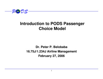
Structured Fares¼Q¼Q¼Q 4Q 2Q 1.5 Q13
¼Q¼Q¼Q 4Q 2Q 1.5 Q14
Interpretation of Cost ParametersAssumed MAX PAY values:4 Virtually all business passengers will pay Y fare if necessary4 Most leisure passengers will not buy B, very few will buy MAssumed relative restriction disutility costs:4 Average business passenger finds fares with morerestrictions less attractive4 Even with restrictions, most leisure passengers prefer Q fare15
EXAMPLE: Fare StructureFare PriceCode LevelYMBQAdvance Sat. NightNonPurchase Min. Stay Refundable 800- 400 7 day 300 14 day 200 21 day-YesYesYes16--YesYesChangeFee---Yes
EXAMPLE: Mean Parameter ValuesBUSINESS LEISUREMAX PAY (mean)Relative Costs:Sat. Night Min. StayNon-RefundableChange Fee17 1200 300 450 150 150 350 50 50
Mean Total Fare Product Disutility( Fare Restriction Costs)Fare PriceCode LevelYMBQAdvance BUSINESSLEISUREPurchase PASSENGERS PASSENGERS 800- 400 7 day 300 14 day 200 21 day 800 850 900 95018 800 750 700 650
Total Disutility Costs Passenger path choice criteria: Least total cost4 Total cost Fare Restriction disutility PQI disutility Replanning disutility Unfavorite airline disutility Impact of passenger disutilities4 With passenger disutility costs included in PODSsimulations, passengers are able to differentiate the“attractiveness” of each path/fare combination, resulting inhigher preference for “favorable” paths19
Other Disutility Costs PQI disutility cost4 Unit PQI disutility cost determined as function of market basefares4 PQI: 1 for nonstop path, 3 for connecting path4 PQI disutility cost Unit PQI disutility cost*PQI Replanning disutility cost4 Applies when a given path is outside of passenger’s decisionwindow4 Function of market basefares Unfavorite airline disutility cost (not used in ePODS)4 Applies when a given path is not a favorite airline4 Function of market basefares20
PODS replicates airline RM system actions over time, taking into account previous interventions: 4Previously applied booking limits affect actual passenger loads and, in turn, future demand forecasts “Historical” booking data is used to generate forecasts for “future” departures. RM system only use