Transcription
Choice Based Conjoint Analysis: Discrete ChoiceModels vs. Direct Regression?Bilyana Taneva1 , Joachim Giesen2 , Peter Zolliker3 , and Klaus Mueller41Max-Planck Institut für Informatik, GermanyFriedrich-Schiller Universität Jena, Germany3EMPA Dübendorf, Switzerland4Stony Brook University, USA2Abstract. Conjoint analysis is family of techniques that originated inpsychology and later became popular in market research. The main objective of conjoint analysis is to measure an individual’s or a population’spreferences on a class options that can be described by parameters andtheir levels. We consider preference data obtained in choice based conjoint analysis studies, where one observes test persons’ choices on smallsubsets of the options. There are many ways to analyze choice based conjoint analysis data. Here we want to compare two approaches, one basedon statistical assumptions (discrete choice models) and a direct regression approach. Our comparison on real and synthetic data indicates thatthe direct regression approach outperforms the discrete choice models.1IntroductionConjoint analysis is a popular family of techniques mostly used in market research to assess consumers’ preferences, see [4] for an overview and recent developments. Preferences are assessed on a set of options that are specified by multiple parameters and their levels. In general conjoint analysis comprises two tasks:(a) preference data assessment, and (b) analysis of the assessed data. Commonto all conjoint analysis methods is that preferences are estimated from conjointmeasurements, i.e., measurements taken on all parameters simultaneously.Choice based conjoint analysis is a sub-family of conjoint analysis techniquesnamed after the employed data assessment/measurement method, namely a sequence of choice experiments. In a choice experiment a test person is confrontedwith a small number of options sampled from a parametrized space, and has tochoose his preferred option. The measurement is then just the observation of thetest person’s choice. Choice based conjoint analysis techniques can differ in theanalysis stage. Common to all methods is that they aim to compute a scale onthe options from the assessed choice data. On an ordinal scale that is a rankingof all the options, but more popular is to compute an interval scale where anumerical value, i.e., a scale value, is assigned to every option. The interpretation is, that an option that gets assigned a larger scale value is more preferred.?Joachim Giesen and Peter Zolliker were partially supported by the Hasler Stiftung(Proj. #2200).
Differences of scale values have a meaning, but there is no natural zero. Thatis, an interval scale is invariant under translation and re-scaling by a positivefactor.The purpose of our paper is to compare two analysis approaches on measuredand synthetic data. Both approaches compute an interval scale from choice data.The first approach builds on probabilistic modeling and can be seen as an extension of the popular discrete choice methods, see for example [7], to the case ofconjoint measurements. The second approach is direct regression introduced byEvgeniou, Boussios and Zacharia [2] that builds on ideas from maximum marginclassification aka support vector machines (though applicability of the kerneltrick, which mostly contributed to the popularity of support vector machines,seems not so important for conjoint analysis). We also study a geometricallyinspired direct regression approach based on computing the largest ball that canbe inscribed into a (constraint) polytope. Both approaches, i.e., discrete choicemodels and direct regression, can be used to compute the scale for either a population of test persons from choice data assessed on the population, or for anindividual solely from his choice data. There is also a third option, namely tocompute the scale for an individual from his choice data and the population dataweighted properly. Here we are not going to discuss this third option.2NotationFormally, the options in the choice experiments are elements in the Cartesianproduct A A1 . . . An of parameter sets Ai , which in general can be eitherdiscrete or continuous—here we assume that they are finite. The choice dataare of the form a b, where a (a1 , . . . , an ), b (b1 , . . . , bn ) A and a waspreferred over b by some test person in some choice experiment. Our goal is tocompute an interval scale v : A R on A from a set of choice data.Often it is assumed that the scale v is linear, i.e., that it can be decomposedasn Xvi (ai ),v(a) v (a1 , . . . , an ) i 1where vi : Ai R. In the case of continuous parameters Ai the linearity of thescale is justified when the parameters are preferentially independent, for detailssee [5]. For finite parameter sets linearity still implies preferential independence,but the reverse is in general not true anymore. Nevertheless, in practice linearityis almost always assumed. Also the two methods that we are going to discusshere both assume linearity of the scale1 . The discrete choice models approachfirst estimates the scales vi from the choice data individually first and thencombines them in a second step. Note that the choice data are obtained fromconjoint measurements, i.e., choices among options in A and not in Ai . The directregression (maximum margin or largest inscribed ball) approach estimates the1The linearity assumption can be mitigated by combining dependent parameters intoa single one, see [3] for a practical example.
scales vi simultaneously from the choice data. Note that both approaches haveto estimate the same number of parameters, namely all the values vi (a), a Ai , i 1, . . . , n.3Discrete Choice ModelsDiscrete choice models deal with the special case of a single parameter, i.e., ina sense the non-conjoint case. Let the finite set A denote this parameter set.Choice data are now of the form a b with a, b A and the goal is to computev : A R or equivalently {va v(a) a A}. Discrete choice models make theassumption that the observed choices are outcomes of random trials: confrontedwith the two options a, b A a test person assigns values ua va a andub vb b , respectively, to the options, where (the error terms) a and b aredrawn independently from the same distribution, and chooses the option withlarger value. Hence the probability pab that a is chosen over b is given aspab P r[ua ub ] P r[va a vb b ] P r[va vb b a ]Discrete choice models can essentially be distinguished by the choice of distribution for the a . Popular choices are normal distributions (Thurstone’s (probit)model [6]) or extreme value distributions (Bradley-Terry’s (logit) model [1]), seealso [7]. The values va can be computed for both models either via the differenceva vb from the probability pab which can be estimated by the frequency fabthat a was preferred over b in the choice experiments, or computationally moreinvolved by a maximum likelihood estimator. Here we introduce a least squaresapproach using the frequency estimates for the pab .3.1Thurstone’s Model (probit)In Thurstone’s model [6] the error terms a are drawn from a normal distributionN (0, σ 2 ) with expectation 0 and variance σ 2 . Hence the difference b a is alsonormally distributed with expectation 0 and variance 2σ 2 and hencepab P r[ua ub ] P r[ b a va vb ] Z va vbx2va v b1 e 4σ2 dx Φ, 2σ4πσ 2 where Φ is the cumulative distribution function of the standard normal distributionZ x21e y /2 dy.Φ(x) 2π This is equivalent to va vb 2σΦ 1 (pab ).Using the frequency fab that a was preferred over b (number of times a waspreferred over b divided by the number that a and b have been compared) weset vab 2σΦ 1 (fab ).
3.2Bradley-Terry’s Model (logit)In Bradley-Terry’s model [1] the error terms a are drawn from a standard Gumbel distribution, i.e., the distribution with location parameter µ 0 and scaleparameter β 1. Since the difference of two independent Gumbel distributedrandom variables is logistically distributed we havepab P r[ua ub ] P r[ b a va vb ]eva vbeva1 . 1 eva vbe va e vb1 e (va vb )This impliese vapab ,e vb1 pabwhich is equivalent to va vb lnpab1 pab .Analogously to what we did for Thurstone’s model we set fabvab ln.1 fab3.3Computing Scale ValuesFrom both Thurstone’s and Bradley-Terry’s model we get an estimate vab forthe difference of the scale values va and vb . Our goal is to estimate the va ’s(and not only their differences). This can be done by computing va ’s that bestapproximate the vab ’s (all equally weighted) in a least squares sense. That is, wewant to minimize the residualnXr(va a A) (va vb vab )2 .a,b A;b6 aA necessary condition for the minimum of the residual is that all partial derivatives vanish, which gives r 2 vaX(va vb vab ) 0.b A;b6 aHence A va XXvb b Avab .b A;b6 aSince we aim for an interval scale we can assume thatvalues that minimize the residual are given asva 1 A Xb A;b6 avab .Pb Avb 0. Then the
We can specialize this now to the discrete choice models and get for Thurstone’smodel 2σ Xva Φ 1 (fab ), A b A;b6 aand for Bradley-Terry’s modelva 3.41 A X lnb A;b6 afab1 fab .Multi-parameter (conjoint) caseNow we turn to the multi-parameter case where the options are elements inA A1 . . . An . We assume a linear model and describe a compositionalapproach to compute the scales for the parameters Ai . In a first step we computescales vi using a discrete choice model for the one parameter case, and then ina second step compute re-scale valuesPwi to make the scales vi comparable. Ournfinal scale for A is then given as v i 1 wi vi , i.e.,n Xv (a1 , . . . , an ) wi vi (ai ).i 1To compute the scales vi we make one further assumption: if a (a1 , . . . , an ) Ais preferred over b (b1 , . . . , bn ) A in a choice experiment we interpret thisas ai is preferred over bi to compute the frequencies fai bi . If the parameter levels in the choice experiments are all chosen independently at random, then thefrequencies fai bi should converge (in the limit of infinitely many choice experiments) to the frequencies that one obtains in experiments involving only a singleparameter Ai .To compute the re-scale values wi we use a maximum margin approach (essentially the same approach that was introduced by Evgeniou et. al to computea scale v : A R by direct regression). The approach makes the usual trade-offbetween controlling the model complexity (maximizing the margin) and accuracy of the model (penalizing outliers). The trade-off is controlled by a parameterc 0 and we assume that we have data from m choice experiments available.PnPmminwi ,zj i 1 wi2 c j 1 zjs.t.4Pn wi vi (ai ) vi (bi ) zj 1,if (a1 , . . . , an ) (b1 , . . . , bn ) in the j’th choice experiment.zj 0, j 1, . . . , mi 1Direct RegressionThe regression approach that we described to compute the re-scale values fordiscrete choice models can be also applied directly to compute scale values. Westart our discussion again with the special case of a single parameter, where wehave to estimate va v(a) for all a A.
4.1Single Parameter CaseThe naive approach to direct regression would be to compute scale values va Rthat satisfy constraints of the form va vb 0 if a A was preferred over b Ain a choice experiment. The geometric interpretation of this approach is to picka point in the constraint polytope, i.e., the subset of [ l, l] A for sufficientlylarge l that satisfies all constraints. There are many such points that all encodea ranking of the options in A that complies with the constraints. Since we haveonly combinatorial information, namely choices, there is no way to distinguishamong the points in the constraint polytope—except we have contradictory information, i.e., choices of the form a b and b a which render the constraintpolytope empty. We will have contradictory information, especially when we assess preferences on a population, but also individuals can be inconsistent in theirchoices. It is essentially the contradictory information that makes the probleminteresting and justifies the computation of an interval scale instead of an ordinal scale (i.e., a ranking or an enumeration of all partial rankings compliantwith the choices) from choice information. The choice information now can nolonger be considered purely combinatorial since also the frequency of a b forall comparisons of a and b will be important. To avoid an empty constraintpolytope we introduce a non-negative slack variable zj for every choice, i.e.,va vb zj 0, zj 0 if a was preferred over b in the j’th choice experiment.Now the constraint polytope Pwill always be non-empty and it is natural to aimkfor minimal total slack, i.e., j 1 zj if we have information from m choice experiments. But since va constant for all a A is always feasible we get theoptimal solutionmXva constant, andzj 0.j 1To mitigate this problem we demand that the constraints va vb zj 0 if a bin the j’th choice experiment a should be satisfied with some confidence margin,i.e., the constraints get strengthened to va vb zj 1. Finally, as we didwhen computing re-scale values for discrete choice models we control the modelcomplexity by maximizing the margin. That is, we end up with the followingoptimization problem for direct regression of scale values:PPmminva ,zj a A va2 c j 1 zjs.t.4.2va vb zj 1,if a b in the j’th choice experiment.zj 0, j 1, . . . , mConjoint CaseNow we assume again A A1 . . . An . Of course we could proceed as for thediscrete choice models and re-scale scales computed with direct regression forthe different parameters Ai , but we can also use direct regression to compute
all scale values simultaneously. With a similar reasoning as in for the singleparameter case we obtain the following optimization problem:Pn PPmminvi (a),zj i 1 a Ai vi (a)2 c j 1 zjPni 1 vi (ai ) vi (bi ) zj 1,if (a1 , . . . , an ) (b1 , . . . , bn ) in the j’th choice experiment.zj 0, j 1, . . . , ms.t.4.3Largest Inscribed BallFor the conjoint case we also study a geometrically inspired direct regressionapproach, namely computing the largest ball inscribed into the polytope definedby the constraintsnXvi (ai ) vi (bi ) 0, if (a1 , . . . , an ) (b1 , . . . , bn ) in a choice experiment.i 1We want to estimate the vi (a) for i 1, . . . , n and allPa Ai . That is, wenwant to estimate the entries of a vector v with m i 1 mi components,where mi kAi k. A choice experiment is defined by the characteristic vectorsχa {0, 1}m , whose i’th component is 1 if the corresponding parameter level ispresent in the option a, and 0 otherwise. The constraint polytope can now bere-written asv t (χa χb ) 0, if a b in a choice experiment,or equivalently v t xab 0, where xab (χa χb ) /kχa χb k.The distance of a point v Rm to the hyperplane (subspace) {v Rm v t xab 0} is given by v t xab . The largest inscribed ball problem now becomes when using the standard trade-off between model complexity and quality of fit on theobserved dataPkmaxv,r,z r c j 1 zjs.t.v t xab r zk , if a b in the j’th choice experiment.zj 0, j 1, . . . , kwhere r is the radius of the ball and c is the trade-off parameter. This is a linearprogram, in contrast to the direct regression approach based on maximizing themargin which results in a convex quadratic program.The largest inscribed ball approach does not work directly. To see this observethat the line v1 v2 . . . vm constant is always feasible. If the feasibleregion contains only this line (which often is the case), then the optimal solutionof our problem would be on this line. A solution v1 v2 . . . vm constanthowever does not give us meaningful scale values. To make deviations from theline vi constant possible we add a small constant 0 to the left hand sideof all the comparison constraints. In our experiments we chose 0.1.
4.4Cross ValidationThe direct regression approaches (and also our re-scaling approach) have thefree parameter c 0 that controls the trade-off between model complexity andmodel accuracy. The standard way to choose this parameter is via k-fold crossvalidation. For k-fold cross-validation the set of choice data is partitioned intok partitions (aka strata) of equal size. Then k 1 of the strata are used tocompute the scale values, which can be validated on the left out stratum. Forthe validation we use the scale value to predict outcome in the choice experimentsin the left-out stratum. Given v(a) and v(b) for a, b A such that a and b havebeen compared in the left-out stratum, to predict the outcome one can eitherpredict the option with the higher scale value, or one can make a randomizedprediction, e.g., by using the Bradley-Terry model: predict a with probabilityev(a) / ev(a) ev(b) . The validation score can then either be the percentage ofcorrect predictions or the average success probability for the predictions. Forsimplicity we decided to use the percentage of correct predictions.5Data SetsWe compared the different approaches to analyze choice based conjoint analysisdata on two different types of data sets: (a) data that we assessed in a largeruser study to measure the perceived quality for a visualization task [3], and (b)synthetic data that we generated from a statistical model of test persons. So letus describe the visualization study first.5.1Visualization StudyThe purpose of volume visualization is to turn 3D volume data into images thatallow a user to gain as much insight into the data as possible. A prominent example of a volume visualization application is MRI (magnetic resonance imaging).Turning volume data into images is a highly parametrized process among themany parameters there are for example(1) The choice of color scheme: often there is no natural color scheme for thedata, but even when it exists it need not best suited to provide insight.(2) The viewpoint: an image is a 2D projection of the 3D data, but not all suchprojections are equally valuable in providing insights.(3) Other parameters like image resolution or shading schemes.In our study [3] we were considering six parameters (with two to six levels each)for two data sets (foot and engine) giving rise to 2250 (foot) or 2700 (engine)options, respectively. Note that options here are images, i.e., different renderingsof the data sets.On these data sets we were measuring preferences by either asking for thebetter liked image (aesthetics), or for the image that shows more detail (detail). That is, in total we conducted four studies (foot-detail, foot-aesthetics,
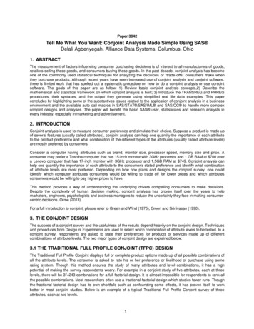
engine-detail, and engine-aesthetics). We had 317 test persons for the two details question studies and 366 test persons for the aesthetics studies, respectively.In each study the test persons were shown two images from the same category,i.e., either foot or engine, rendered with different parameter settings and askedwhich of the two images they prefer (with respect to either the aesthetics or thedetails question). Hence in each choice experiment there were only two options,see Figures 1 and 2 for examples.Fig. 1. Data set foot: Which rendering do you like (left or right)?Fig. 2. Data set engine: Which rendering shows more detail (left or right)?In [3] we evaluated the choice data using the Thurstone discrete choice modelfor the whole population of test persons. There we used a different method tore-scale the values from the first stage than described here. The method we usedis based on the normal distribution assumption and thus not as general as themethod described here.
5.2Synthetic DataWe were also interested to see how well the different methods perform when weonly use information provided by a single person. Unfortunately the informationprovided individually b
Conjoint analysis is a popular family of techniques mostly used in market re-search to assess consumers’ preferences, see [4] for an overview and recent devel-opments. Preferences are assessed on a set of options that are speci ed by multi-ple parameters and their levels. In genera