Transcription
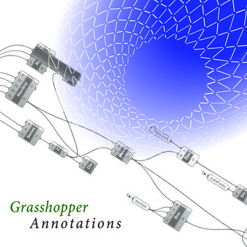
GrasshopperAnnotations
Contributors:Andrew PayneRajaa IssaZubin KhabaziKyle TalbottAll rights reserved. No part of this book may be reproducedin any form by any electronic or mechanical means (includingphotocopying, recording, or information storage and retrieval)without permission in writing from the publisher.While every effort has been made to contact copyright holdersfor their permission to reprint material in this book, thepublisher would be grateful to hear from any copyright holderwho is not acknowledged here and will undertake every effortto rectify any errors or omissions in future editions.Written and produced for Independent Study with the HonorsCollege and the School of Architecture and UrbanPlanning at the University of Wisconsin, Milwaukee.July 2010Verge Domain PublishingAll rights reservedKevin Hinz6068 Templeton DriveWaunakee, WI 53597 USAkevin h us@yahoo.comISBN 978-0-578-07439-9Grasshopper AnnotationsCopyright 2010 Kevin Hinz
Thank you to the SARUP students and professors who providedadvice and analysis during the planning, development andexecution of the following work. I appreciate your help, patienceand the assistance provided to write the following scripts.Special thanks to Andrew Payne, Rajaa Issa, Zubin Khabaziand Kyle Talbott for making their intellectual property availablefor annotation.Kevin Hinzkevin h us@yahoo.com
Contentsch 1 Spacial Orientation6ch 2 Matrix and Attractors10ch 3 Conditional Statements14ch 4 Curves, Lines and Data Management20ch 5 Exporting Data26ch 6 Vector Relationships30ch 7 Curves and Surfaces38ch 8 Spiraled Matrices44foot notes 50references 51
1IntroductionParametric NotationThis publication is assembled as an elaboration of exercises provided in Andrew Payne and Rajaa Issa’s GrasshopperPrimer. In addition, lessons outlined in Algorithmic Modeling with Grasshopper by Zubin Khabazi, are referenced as well asscripts written for studio projects during Professor Kyle Talbott’s Microcosm Studio. The goal is to provide information andinsight encountered while completing the Grasshopper tutorials with intention to share the experiences encountered duringthe learning process.Grasshopper is an intuitive parametric modeling plug-in running on the Rhinoceros platform. As with any new learningexperience, prior education and explanation is paramount to knowledge retention. So much knowledge is available thatit can be difficult to discern the exact solution and come away with specific information. This publication is probablyno different. However, as an addition to the extensive work assembled by the afore mentioned authors, GrasshopperAnnotations brings analysis to the table during the administration of tutorials. Explanations provided in the accompanyingsource files provide insight into the interface organization as well as a breakdown outlining design intentions and how theyrelate to the construction of each script. Throughout the course of the book and dvd, you will find suggestions and solutionsto potential problems for peculiar encounters. I encourage readers to include their own notes at the conclusion of eachchapter to share additional acquired experiences.Because dates are significant factors to the evolutionary progression of changing programs and the information thataccompanies them, each of the source files corresponding to the following chapters have been dated. Links to the toolsused to construct and assemble this publication are available in the dvd accompanying the printed work and also listed inthe bibliography in the conclusion of this document. Other time sensitive specifications, outlining exterior works cited andprograms used are as follows:Rhinoceros 4.0, SR7 ownload/Grasshopper Plugin version 0.6.0059 opper Primer for version 0.6.0007, tive Algorithms using Grasshopper, er/1.0/docs/en/Generative%20Algorithms.pdfNote: recent versions of Grasshopper often develop issues that prevent the use of scripts written on previous versions. Onesuch encounter happened during the production of this publication because I updated to plugin version 0.6.0055 whileworking; the issue was minor. The most recent current stable Grasshopper build is now 0.6.0059 but development is tobuild 0.7.0036 as of July, 2010.6
7
2Spacial OrientationDraw a Parametric BoxThis exercise provides an introduction to thecreation and subsequent manipulation of basicgeometry. Although the exercise appears at firstelementary, the theory behind what is occurring haspowerful potential.I recommend exploring the theories presented hereas a way to practice and thus grasp how geometryis determined from spacial orientation.source files801 BasicGeometry31Jan2010 spacialOrientation KevinHinz.3dm31Jan2010 spacialOrientation KevinHinz.ghx
2The definition below uses anarray of points from Rhino toform the base of the box. Notehow Grasshopper interacts withthe persistent data in Rhino todevelop a parametric series ofcrosses dependent on the inputparameters.9
11Spacial OrientationA multitude of component choices provide numerousways to assemble data. At left, the orientatingpoints lines are shown in green to highlight the boxboundaries. Note in the source file how points canboth be used to determine the corners of the boxand be derived from the box as separate entities.Once other exercises are mastered, the re-usedgeometry can be reassembled into more complexforms . For example, a simplified version of abovecould be a column based on a point grid fromchapter 3, Matrix and Attractors. Thus, all columnswould act together according to the specificationsset here.1source files1001 BasicGeometry31Jan2010 spacialOrientation KevinHinz.3dm31Jan2010 spacialOrientation KevinHinz.ghx
Notes:See also ch. 11 in the Grasshopper Primerfor more complex applications1111
21Matrix and AttractorsSeries , Range and AttractionHere, the operator has an opportunity to investigate the orientation of the regular grid.Again, complexity is kept to a minimum but as in chapter 1, understanding simpleorganizational patterns is a preemption to understanding more complex algorithmicorganization; a strong foundation of knowledge is required for success.When working with the Grasshopper files provided, use the preview mode to limitvisible data for each of the included four definitions: Attractor Lines, Point Lists andCurves, Point Grids (Matrix), and Attractors, point list display.Attractor Lines explore the Range component to draw a basic grid. Range is used asa uniform multiplier to repeat data in a regular pattern. Its location in the Grasshopperinterface (Logic / Sets / Range) is rooted in the description of its function (a logicaluniform set of repeatable data inputs). As you may well be aware, Grasshoppercomponents are organized intuitively according to their functional capabilities. Practiceand experience will strengthen your navigation skills within the program.The chapters Point Lists and Curves help layout the order behind data lists and curvelists while Point Grids explore the Series. Series allows the introduction of complexityto the ordering system requiring three inputs: first number, step size and number ofvalues; repetitive generation of data can be easily controlled.source files1202 Matrix and Attractors03Feb2010 PointMatrix KevinHinz.3dm03Feb2010 PointMatrix KevinHinz.ghx
2figure 01persistent data assignmentIn figures 01 and 02, volatile data(geometry in Grasshopper) isworking congruently with persistentdata (geometry in Rhino). Whenchanges are made in Rhino tothe assigned point locations,the volatile data is automaticallyupdated to represent the relativerelationship.figure 0213
12Matrix and AttractorsInterval is utilized to set up parametersfor a subsequent point grid (in green)that exists within a defined domain.Note that a name change has occurredduring production of the plug-in: whatwas “Interval” previously, is nowtitled “Domain.” Notation and logicalexplanation of the change can be foundin the .ghx file.This definition combines volatile andpersistent data resulting in a frame workthat can be utilized as an organizationalsystem for parametrically complexdesigns.source files1402 Matrix and Attractors03Feb2010 PointMatrix KevinHinz.3dm03Feb2010 PointMatrix KevinHinz.ghx
Notes:215
31Conditional StatementsGeometric EvaluationConditional Statements are one of the most powerfultransformation tools available in scripting. Thinkof it as a set of emergency instructions to beinitiated when a predetermined variable reaches apredetermined size. Combine this statement withreoccurring or repetitive computative data and youcan often produce unexpected geometry.The exercises represented here and in chapter 7of the Grasshopper Primer explore input / outputrelationships: one of the strongest core potentialsof parametric design. Combining the Series andRange components from exercise 2 with conditionalstatements assists design development that isdependent upon object size, physical space locationand designer intent.As before, this exercise is simple; the notatedexplanation is even less complex. It is up to theuser to implement the tools presented.source files1603 ConditionalStatements05Feb2010 spacialOrientation KevinHinz.3dm05Feb2010 spacialOrientation KevinHinz.ghxfigure 04
3As a conditional statement, Dispatch (figure 03) isused to evaluate incoming data lists. Its location,Logic / List / Dispatch, describes its function. Inthis example, when the variableX 25 false, thepolygon is centered at the left plane, consequently,if variableX 25, the polygon shifts to the rightplane (figure 04).To introduce complexity, the script below draws apolygonal shape that shares its number of sideswith the its radius in integers (figure 05). A circlecircumscribes the polygon having an similar radius.Note the polygon’s radius input and the circle’sinput come form the same source; each isdependent on the other.figure 03figure 0517
13Conditional StatementsEach component requires specific types of data for input:either integers (whole numbers) or doubles (decimalnumbers). You should be familiar with them by now.Because the number of sides on a polygon must be aninteger, Grasshopper converts the decimal to the nearestwhole number while leaving the radius as determined. Notethe images above.source files1803 ConditionalStatements05Feb2010 spacialOrientation KevinHinz.3dm05Feb2010 spacialOrientation KevinHinz.ghxNot utilized here is the Rf input, or corner fillet radius.By combining any one of a number of equations, it wouldbe easy to derive an inputvalue dependent on variableX.Definitions often produce themost interesting results whengeometry is built slowly, uponitself. Simple actions work asinstructions in a recipe.
3The illustration below shows a trianglehaving a radius of 3.38 units circumscribedby a circle sharing the same radius.variableX is converted to the nearestinteger, 3.At right, the radius and polygon sides areidentical to draw a dodecagon.19
13Theorysource files2003 ConditionalStatements05Feb2010 spacialOrientation KevinHinz.3dm05Feb2010 spacialOrientation KevinHinz.ghx
Notes:321
4Curves, Lines and Data ManagementSpiral CurvesDetailed instructions of this exercise can be found inchapter 7.4 of the Grasshopper Primer - Functions& Numeric Data. The ability of Grasshopperto transpose and manipulate data into threedimensions is most astounding. This exercise setsup a framework of points that can be used in avariety of different applications. A curve drawnthrough the point list provides a visual reference tothe structure of the list.Once achieved, the points could be referencesfor more complex geometry or manipulated intoan organizing structure with more elegant forms. Isuggest exploring this example further by introducingthe Pipe or Loft Surface components.At right, the functions x*sin(5*x) and x*cos(5*x)are used to generate x and y point coordinates;the same Range input, when introduced as the zinput, lifts the spiral into 3 dimensions. Note howthe points appear to be organized around the curve(in actuality, the curve is drawn through the pointlist). As the number of points in within the Rangeis increased, the list begins to take on a complexstructure; depth can be achieved that has potentialto manipulate a viewers perspective of the pattern.source files2204 CurvesLinesData13Feb2010 Functions KevinHinz.3dm13Feb2010 Functions KevinHinz.ghx
4Above and at left iterate the numerous trigonometriccomponents available in the Grasshopper library.Easy to find and drag onto your canvas, thisexercise is best learned by exploring; I wouldsuggest building a similar model as above andmanipulating the wavelength, frequency andamplitude parameters to grasp how each operatoreffects the volatile data. Here you will be introducedto graphs. Graphs can be difficult to understand dueto the nature of trigonometry but they can act as afast and powerful tool to manipulate geometry.source files04 CurvesLinesData14Feb2010 TrigometricCurves KevinHinz.3dm14Feb2010 TrigometricCurves KevinHinz.ghxSince the creation of this file, ArcCosine, ArcSineand ArcTangent have been added to the mostrecent release of Grasshopper; they produce somewidely unexpected results as well.23
14Curves, Lines and Data ManagementThe Sort component is one of the most powerfultools used to manage data in Grasshopper. Thecomponent is found in the Logic panel under List,as is most all of Grasshopper’s list managementcomponents. The definition exemplified ordersa group of circles placed randomly with randomradii according to radius and circumference. In thesource file listed below, you will find additional datamanipulation tools such as List, Shift, Cull, Weave,Flatten and many more. Their value will becomemore evident near the conclusion of this manual.Authors Payne and Rajaa Issa included aninformative drawing created by David Rutten tographically represent the way Grasshopper managesdata ; I need not repeat it here. Essentially, datapaths are managed much like the trunk of a treewhereas each branch may be subdivided, shearedand / or grafted to additional data structures. Asmore information is stored, such as point locationsand line lengths, paths and numbers are linkedand woven together into sub branches, sub-subbranches and so on. Grasshopper makes it easyto view and manipulate data streams as definitionsbecome more complex.2Chapters 8.1, 8.2 and 8.3 of the GrasshopperPrimer provide very informative definitions for keylist management components. Observation is keyto interpreting the resulting output. See the sourcefile listed below left for detailed illustrations andobservations of data found in the yellow read outpanels, such as those seen at right, and the sourcefile (next page) for notation about shifting data. Shiftworks to take one or more lists and move volatiledata according to the input value (in integers); it isas if you simply twist the list as desired.source files2404 CurvesLinesData14Feb2010 DataManagment KevinHinz.3dm14Feb2010 DataManagment KevinHinz.ghx
4source files04 CurvesLinesData23Feb2010 shiftingData KevinHinz.3dm23Feb2010 shiftingData KevinHinz.ghx25
14Theorysource files2604 CurvesLinesData13Feb2010 Functions KevinHinz.3dm13Feb2010 Functions KevinHinz.ghx14Feb2010 TrigometricCurves KevinHinz.3dm14Feb2010 TrigometricCurves KevinHinz.ghx14Feb2010 DataManagment KevinHinz.3dm14Feb2010 DataManagment KevinHinz.ghx23Feb2010 shiftingData KevinHinz.3dm23Feb2010 shiftingData KevinHinz.ghx
Notes:See chapter 8 in the Grasshopper Primer4227
5Exporting rom Grasshopper to ExcelData produced in Grasshopper can often times be analyzed and utilizedby other software packages such as Microsoft’s Excel. Spread sheets arevery functional documents, able to tabulate material quantities, produceproject estimates and calculate costs. In addition, data exports, suchas x, y, z coordinates, can be read by robotic arms to place materials.Original source files are listed below however, I recommend using theGrasshopper Primer to build your own from scratch; the exercise issimple. If you are looking for more challenging tutorials, look to ZubinKhabazi’s Algorithmic Modeling, chapter 8 Fabrication.Page 1In the upper right image, this page, you will see a graph mapper attachedto a display panel; note the exported data at left from the .csv streamfile. Near right you are the line lengths and start point locations for thecolumnar structure on the next page. My experiences with exportingdata were more successful to Microsoft’s Excel than the OpenOffice’sCalc. The interface appears more friendly in Microsoft and the linked filesreadily update and reload with ease.source files2805 DataCommunication24Feb2010 ExportingData KevinHinz.3dm324Feb2010 ExportingData KevinHinz.ghxSheet1Line(L:52.863312 in)Line(L:52.863313 in)Line(L:52.863312 in)Line(L:52.863313 in)Line(L:52.863312 in)Line(L:52.863313 in)Line(L:52.863313 in)Line(L:52.863313 in)Line(L:52.863313 in)Line(L:52.863313 in)Line(L:52.863312 in)Line(L:52.863312 in)Line(L:52.863312 in)Line(L:52.863313 in)Line(L:52.863312 in)Line(L:52.863312 in)Line(L:52.863313 in)Line(L:52.863313 in)Line(L:52.863313 in)Line(L:52.863313 in)Line(L:52.863313 in)Line(L:52.863313 in)Line(L:52.863313 .0}0.0}0.0}0.0}
5The columnar structure is used to iterate the export process; better resolution is found in the source filebut I recommend completing the process on your own. Essentially, this exercise explores the use ofspreadsheets. The only thing new in Grasshopper is to choose the stream content selection with a rightmouse over the panel display: that easy.29
15Theorysource files3005 DataCommunication24Feb2010 ExportingData KevinHinz.3dm324Feb2010 ExportingData KevinHinz.ghx
Notes:3see also the .csv files for streamed data output531
6Vector RelationshipsDistance FactorsUnderstanding vector is crucial to building mostanything with Grasshopper. Vectors have an origin,orientation and a magnitude, three things needed tocreate parametric proximity relationships.The image at right, below, illustrates an attractorscript build from a point grid and series of circles.Each radius is adjusted according to the distancebetween a circles center point and two chosenreaction points . The number of reaction points iseasily modifiable as is the reaction point itself.For example, if one wanted a curve to be inflectionalgeometry, you would need to establish a point onthat curve to measure to. Thus, you would need aclosest point on curve component (Crv CP) shownbelow.4In either case, the logic behind the attractor script issimple:-create a point grid to draw some modifiable shape-assign some form of attractor-evaluate a distance to the attractor-introduce a user defined variable to control the rate of influence-insert a minimum or maximum cut off to control shape size-draw shape according to determined distance parametersAttractor scripts can be powerful tools to create gradientgeometrical forms; none would be possible without the vector:origin, orientation and magnitude.source files3206 VectorBasics24Feb2010 Vectors101 KevinHinz.3dm24Feb2010 Vectors101 KevinHinz.ghx
6The example above shows howan attractor can be appliedto a three dimensional form.While nearly identical to theprevious exercise, the script tothe right draws geometry first,then magnifies it according tothe distance between its centerand the attractor .5Here, scalar computation isalso applied to object coloring.source files06 VectorBasics06Mar2010 ScalarColor KevinHinz.3dm06Mar2010 ScalarColor KevinHinz.ghxoriginal geometry33
16Vector RelationshipsSort componentThe Sort component becomes critical when applying the color gradient.Input items represent the scaled distances between matrix points andthe attractor point; the values are ordered according to its position in thematrix. Because we want the color to be graduated according to distance,values must be reordered. If Sort is removed from the equation, and thefirst and last list items inputted directly into the shader, only the cubes onthe extremities show a color gradient; the data is ordered in very much ina different way.Note that because the color gradient is determined by the attractor, andnot the cube, it operates as its own system.source files3406 VectorBasics06Mar2010 ScalarColor KevinHinz.3dm06Mar2010 ScalarColor KevinHinz.ghx
Vector Relationships6The real power of computationis demonstrated at right.Highlighted in green, threevery different curves are usedto demonstrate the script’sversatility. A 1/4” squareis attached to the end of a1/4” line which is orientatedperpendicular to the desiredcurve .6Where it would take countlesshours of applying geometrictheory, once built, the script willaccomplish in seconds.Computation and MaterialThe bridge model above is design by conventionalmeans but manufactured with scripting. A simpleconnection (below) was uncovered during materialexploration; Grasshopper was used to apply thezipper connection to irregular surface edges anddevelop refined curves for an elegant structure flow.Conventional modeling tested the design, digitalmodeling clarified the planand scripting applied thegeometrical frameworkto polish the layout andsimplify the constructionprocesses. The finalapplication and productionof the model would beintensely laborious.Following the connection discovery, manual iterations exploring widthand degree of curvature (in bridge components) produced variationsin bridge formation. Final iterations were used as templates for pointparameters then refined with Grasshopper’s Bezier Spline component.Final bridge component parameterswere documented for explanationpurposes but design approximationsare completed manually. The projectdemonstrates how conventionalmodeling technics can be combinedwith digital modeling and scripting toproduce a comprehensive project.[Academic use only]source files06 VectorBasicszipperConnection22Feb2010 BridgeConnection KevinHinz.3dm22Feb2010 BridgeConnection KevinHinz.ghxsee the source file and page 34 for a detailedaccount of the logic635
16Vector Relationshipsfigure 07figure 09see figure 15,next pagelength valueinserted heresee figure 14,next pagelength computationfigure 06: divide any curve accordingto length between divisionsDivide: Logic - Curve - Divisionfigure 07: display tangent vectorat division pointDisplay: Vector - Vectorfigure 08: rotate above vectorto perpendicularRotate: XForm - Euclidianfigure 09: get vector used to moveframe for polygon centerMove: XForm - Euclidianfigure 10: moved framefigure 11: vector showingframe centerfigure 12: final rotated framefigure 06source files3606 VectorBasicszipperConnection22Feb2010 BridgeConnection KevinHinz.3dm22Feb2010 BridgeConnection KevinHinz.ghxfigure 08figure 10figure 12figure 11A simple series of steps organize the applicationof this “zipper”-like definition: divide a lineaccording to length / get a line perpendicularto the tangent at each division point / placea square at the end of the perpendicular line.Placing the square proves to be the mostcomplex; Grasshopper draws polygons fromtheir center, in a diagonal rather than from thecenter by their side edge. More than 50% of thescript (and 75% of the time it took to write) isdedicated to drawing the square polygon.Because Grasshopper is organized logically,components are easy to find, if you know whatyou want to do and what the mathematical theoryis behind the transformation. Note the lengthcomputation at the beginning of the script; thedefinition expresses the Pythagorean Theoremand how the location (listed under the figuredescriptions at left) is directly related to how thecomponent functions.
6figure 13Figure 13, found in the source file listedbelow, illustrates how the definition wastransformed according to the script’sapplication. Small changes, such asthe rotation reversal shown in figure 14,modify the zippers’ orientation accordingto the designer’s desire (shown aboveat right). Note that Grasshopperrequires the angle of rotation to be inRadians, hence, the Pi / 2 (or Pi / -2in this example) to rotate thevector 90 degrees. Figure 15illustrates a vector reversal forthe two definitions above at left.figure 14One each of the 4 definitionsabove are used to apply thescript left or right and above orbelow.figure 15source files06 VectorBasicszipperConnection22Feb2010 BridgeConnection KevinHinz.3dm22Feb2010 BridgeConnection KevinHinz.ghx37
16Theorysource files06 VectorBasics24Feb2010 Vectors101 KevinHinz.3dm24Feb2010 Vectors101 KevinHinz.ghx06Mar2010 ScalarColor KevinHinz.3dm06Mar2010 ScalarColor KevinHinz.ghx38zipperConnection22Feb2010 BridgeConnection KevinHinz.3dm22Feb2010 BridgeConnection KevinHinz.ghx
Notes:4see ch 2 of this publication for additional matrixand attractor information5see the source file for detailed explanation ofhow the components operate6see the source file and page 34 for a detailedaccount of the logic639
7Curves and SurfacesCurve TypesYou will find a working model of curve types and degree testsin the source file listed below. Because of its mathematicalcomplexity, I will suggest researching more completeinformation about NURBS curves found athttp://en.wikipedia.org/wiki/NURBS.At right, top, are two drawings; above, you will find a simplecurve with a varying slide parameter attached. Furtherinspection will shed light onto one way curve structure can bemanipulated. The lower, more fanciful curve, is constructedfrom a series of arcs. Because a thorough explanation isprovided, I recommend seeing the Grasshopper Primer,pg. 67 - chapter 10, for detailed description of availablecurve types in Grasshopper.At right, lower, is a testament to intuitive navigation within theGrasshopper interface. Working on a challenge presented bya classmate, we struggled in our attempts to determine thegeometrical relationships required to inscribe a circle withinany triangle. Writing the script in Visual Basic presented thegreatest challenge because the logic required informationregarding how the data was collected. In other words, weneeded to know which edge was orientated which way tomake the set of instructions work. Grasshopper calculatedthis for us. Soon after trying to build the script using primitivegeometric relationships, I uncovered the component InCircle,located at Curve / Primitive / InCircle.Organization of Grasshopper components can be understoodif the analysis of the final geometrical relationship isunderstood; the two go hand in hand.source files4007 Curves and Surfaces06Mar2010 curveTypes KevinHinz.3dm06Mar2010 curveTypes KevinHinz.ghx
7Surface ManipulationsAt first glance, the script at right appears easy tofollow and understand. However, the examplequickly becomes complex to the point of freezingthe CPU used to construct it. Strangely enough,perhaps due to the way Rhino and Grasshoppercompute data, the definition does not overwhelmthe system when assembled from scratch; problemsarise only when tweaking parameters and testingiterations after the script is built. Have patiencewhen investigating this definition.Beginning with three double curves, a surface islofted between before being offset. Examples ofa columnar structure, similar to a peristyle, canbe found in the lower portion of the script. Bycombining a point grid (see following page) with acomplex curve, what is typically a simple organizedstructural system, can easily become somethingmuch more fluid and dynamic.The aim of experimentation outlined in this chapterand the next, point towards a reintroduction ofcomplexity and movement into architecture: twointerjections that have been shunned since thebeginning of the modern movement.source files07 Curves and Surfaces06Mar2010 surfaceRelationships KevinHinz.3dm06Mar2010 surfaceRelationships KevinHinz.ghx41
7Curves and SurfacesAt left, above, you will see the application of apoint grid with a radius controlled circle applied.Form here, the script found in the source file takestwo directions: one to design a set of columnsbetween the complex surface, the other to articulatea uniquely texture surface. Follow the illustrations(and the majority of the definition) for a combinationof the exercises outlined in the chapters presentedso far.At left, center, cones are placed on the point grid.On each cone tip, a plan is used to set up for thespheres shown at left, below. Looking back tochapter 2, this script copies and pastes (ctrl C ,ctrl V) the earlier attractor script to combine andbuild the definition’s complexity.As mentioned earlier, the computation soonchallenges power of standard computers thus,the final component is disabled.source files4207 Curves and Surfaces06Mar2010 surfaceRelationships KevinHinz.3dm06Mar2010 surfaceRelationships KevinHinz.ghx
7Once the final Trim component isenabled (and the computer getsdone thinking.) the individualcones/ unique shape is revealed.Options to further develop andcomplete this design could includeplacing the cones atop the columnsfrom earlier or even joining thecones to your columns andbaking in Rhino before meshing,flattening, cutting and constructinga paper model of the design.Evolution of the idea
This publication is assembled as an elaboration of exercises provided in Andrew Payne and Rajaa Issa's Grasshopper Primer. In addition, lessons outlined in Algorithmic Modeling with Grasshopper by Zubin Khabazi, are referenced as well as scripts written for studio projects during Professor Kyle Talbott's Microcosm Studio.