Transcription
The Fundamental Theorem of Linear AlgebraGilbert StrangThe American Mathematical Monthly, Vol. 100, No. 9. (Nov., 1993), pp. 848-855.Stable URL:http://links.jstor.org/sici?sici CO%3B2-AThe American Mathematical Monthly is currently published by Mathematical Association of America.Your use of the JSTOR archive indicates your acceptance of JSTOR's Terms and Conditions of Use, available athttp://www.jstor.org/about/terms.html. JSTOR's Terms and Conditions of Use provides, in part, that unless you have obtainedprior permission, you may not download an entire issue of a journal or multiple copies of articles, and you may use content inthe JSTOR archive only for your personal, non-commercial use.Please contact the publisher regarding any further use of this work. Publisher contact information may be obtained athttp://www.jstor.org/journals/maa.html.Each copy of any part of a JSTOR transmission must contain the same copyright notice that appears on the screen or printedpage of such transmission.The JSTOR Archive is a trusted digital repository providing for long-term preservation and access to leading academicjournals and scholarly literature from around the world. The Archive is supported by libraries, scholarly societies, publishers,and foundations. It is an initiative of JSTOR, a not-for-profit organization with a mission to help the scholarly community takeadvantage of advances in technology. For more information regarding JSTOR, please contact support@jstor.org.http://www.jstor.orgTue Feb 5 09:12:11 2008
The Fundamental Theorem of LinearAlgebraGilbert StrangThis paper is about a theorem and the pictures that go with it. The theoremdescribes the action of an m by n matrix. The matrix A produces a lineartransformation from R" to Rm-but this picture by itself is too large. The "truth"about Ax b is expressed in terms of four subspaces (two of R" and two of Rm).The pictures aim to illustrate the action of A on those subspaces, in a way thatstudents won't forget.The first step is to see Ax as a combination of the columns ofA. Until then themultiplication Ax is just numbers. This step raises the viewpoint to subspaces. Wesee Ax in the column space. Solving Ax b means finding all combinations of thecolumns that produce b in the column space:1 1 1" 'Columns of A ] x l c o u m n x n o u m nxnThe column space is the range R(A), a subspace of Rm. This abstraction, fromentries in A or x or b to the picture based on subspaces, is absolutely essential.Note how subspaces enter for a purpose. We could invent vector spaces andconstruct bases at random. That misses the purpose. Virtually all algorithms andall applications of linear algebra are understood by moving to subspaces.The key algorithm is elimination. Multiples of rows are subtracted from otherrows (and rows are exchanged). There is no change in the row space. This subspacecontains all combinations of the rows of A, which are the columns of AT. The rowspace of A is the column space R(AT).The other subspace of R" is the nullspace N(A). It contains all solutions toAx 0. Those solutions are not changed by elimination, whose purpose is tocompute them. A by-product of elimination is to display the dimensions of thesesubspaces, which is the first part of the theorem.The Fundamental Theorem of Linear Algebra has as many as four parts. Itspresentation often stops with Part 1, but the reader is urged to include Part 2.(That is the only part we will prove-it is too valuable to miss. This is also as far aswe go in teaching.) The last two parts, at the end of this paper, sharpen the firsttwo. The complete picture shows the action of A on the four subspaces with theright bases. Those bases come from the singular value decomposition.The Fundamental Theorem begins withPart 1. The dimensions of the subspaces.Part 2. The orthogonality of the subspaces.848THE FUNDAMENTAL THEOREM OF LINEAR ALGEBRA[November
The dimensions obey the most important laws of linear algebra:dim R( A ) dim R( AT) and dim R( A ) dim N( A ) n.When the row space has dimension r, the nullspace has dimension n - r.Elimination identifies r pivot variables and n - r free variables. Those variablescorrespond, in the echelon form, to columns with pivots and columns withoutpivots. They give the dimension count r and n - r. Students see this for theechelon matrix and believe it for A.The orthogonality of those spaces is also essential, and very easy. Every x in thenullspace is perpendicular to every row of the matrix, exactly because Ax 0:The first zero is the dot product of x with row 1. The last zero is the dot productwith row m. One at a time, the rows are perpendicular to any x in the nullspace.So x is perpendicular to all combinations of the rows.m e nullspace N( A ) is orthogonal to the row space R( AT).What is the fourth subspace? If the matrix A leads to R(A) and N(A), then itstranspose must lead to R(AT) and N(AT). The fourth subspace is N(AT), thenullspace of AT. We need it! The theory of linear algebra is bound up in theconnections between row spaces and column spaces. If R(AT) is orthogonal toN(A), then-just by transposing-the column space R(A) is orthogonal to the"left nullspace" N ( A ) Look.at y 0:A T [column 1 of Acolumn n of AI y [:I. Since y is orthogonal to each column (producing each zero), y is orthogonal to thewhole column space. The point is that AT is just as good a matrix as A. Nothing isnew, except AT is n by m. Therefore the left nullspace has dimension m - r.ATY 0 means the same as y% OT. With the vector on the left, y% is acombination of the rows of A. Contrast that with Ax combination of thecolumns.The First Picture: Linear EquationsFigure 1shows how A takes x into the column space. The nullspace goes to thezero vector. Nothing goes elsewhere in the left nullspace-which is waiting itsturn.With b in the column space, Ax b can be solved. There is a particularsolution x, in the row space. The homogeneous solutions x, form the nullspace.The general solution is x, x,. The particularity of x, is that it is orthogonal toevery x,.May I add a personal note about this figure? Many readers of Linear Algebraand Its Applications [4] have seen it as fundamental. It captures so much aboutAx b. Some letters suggested other ways to draw the orthogonal subspacesartistically this is the hardest part. The four subspaces (and very possibly the figureitself) are of course not original. But as a key to the teaching of linear algebra, thisillustration is a gold mine. 19931THE FUNDAMENTAL THEOREM OF LINEAR ALGEBRA849
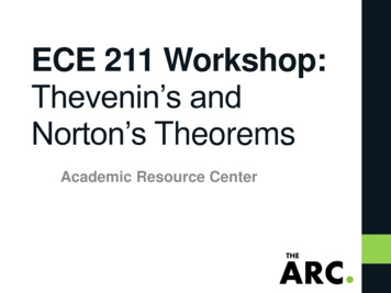
Figure 1. The action of A: Row space to column space, nullspace to zero.Other writers made a further suggestion. They proposed a lower level textbook,recognizing that the range of students who need linear algebra (and the variety ofpreparation) is enormous. That new book contains Figures 1 and 2-also Figure 0,to show the dimensions first. The explanation is much more gradual than in thispaper-but every course has to study subspaces! We should teach the importantones.The Second Figure: Least Squares EquationsIf b is not in the column space, Ax b cannot be solved. In practice we stillhave to come up with a "solution." It is extremely common to have more equationsthan unknowns-more output data than input controls, more measurements thanparameters to describe them. The data may lie close to a straight line b C Dt.A parabola C Dt t would'come closer. Whether we use polynomials orsines and cosines or exponentials, the problem is still linear in the coefficientsC, D, E : CC Dt, b, Dt,C Dt, E t t blC Dt, or b,t ; b,There are n 2 or n 3 unknowns, and m is larger. There is no x (C, D) or (C, D, E ) that satisfies all m equations. Ax b has a solution only when thepoints lie exactly on a line or a parabola-then b is in the column space of the mby 2 or m by 3 matrix A.The solution is to make the error b -Ax as small as possible. Since Ax cannever leave the column space, choose the closest point to b in that subspace. Thispoint is the projection p. Then the error vector e b - p has minimal length.To repeat: The best combination g A.Z is the projection of b onto the columnspace. The error e is perpendicular to that subspace. Therefore e b - Af is inthe left nullspace:xCalculus reaches the same linear equations by minimizing the quadratic Ilb - Ax1l2.The chain rule just multiplies both sides of Ax b by AT.850THE FUNDAMENTAL THEOREM OF LINEAR ALGEBRA[November
The "normal equations" are AT& ATb. They illustrate what is almost invariably true-applications that start with a rectangular A end up computing with thesquare symmetric matrix A%. This matrix is invertible provided A has independent columns. We make that assumption: The nullspace of A contains only x 0.(Then A T h 0 implies xQTAx 0 which implies Ax 0 which forces x 0, soA% is invertible.) The picture for least squares shows the action over on the rightside-the splitting of b into p e.Figure 2. Least squares: R minimizes Ilb - A.111 by solving A T k ATb.The Third Figure: Orthogonal BasesUp to this point, nothing was said about bases for the four subspaces. Thosebases can be constructed from an echelon form-the output from elimination.This construction is simple, but the bases are not perfect. A really good choice, infact a "canonical choice" that is close to unique, would achieve much more. Tocomplete the Fundamental Theorem, we make two requirements:Part 3. m e basis vectors are orthonormal.Part 4 . m e matrix with respect to these bases is diagonal.If v , , . . . , v, is the basis for the row space and u , , . . . , u , is the basis for thecolumn space, then Avi uiui. That gives a diagonal matrix 2. We can furtherensure that ui 0.Orthonormal bases are no problem-the Gram-Schmidt process is available.But a diagonal form involves eigenvalues. In this case they are the eigenvalues ofA% and AAT. Those matrices are symmetric and positive semidefinite, so theyhave nonnegative eigenvalues and orthonormal eigenvectors (which are the bases!).Starting from A%vi u:vi, here are the key steps:oiTA%vi u:v:viAA%vi U;AV so thatSOthatllAvill uiui Avi/ui is a unit eigenvector of AAT.All these matrices have rank r. The r positive eigenvalues u: give the diagonalentries ui of 2.19931THE FUNDAMENTAL THEOREM OF LINEAR ALGEBRA851
The whole construction is called the singular value decomposition (SKI). Itamounts to a factorization of the original matrix A into UCVT, where1. U is an m by m orthogonal matrix. Its columns u,, . . . , u,, . . . , u , are basisvectors for the column space and left nullspace.2. C is an m by n diagonal matrix. Its nonzero entries are a, 0, . . . , a, 0.3. V is an n by n orthogonal matrix. Its columns v,, . . . , v,, . . . , v, are basisvectors for the row space and nullspace.The equations Av, aiui mean that AV UC. Then multiplication by vTgives A U 2 V T .When A itself is symmetric, its eigenvectors ui make it diagonal: A u A u .The singular value decomposition extends this spectral theorem to matrices thatare not symmetric and not square. The eigenvalues are in A, the singular valuesare in 2.The factorization A U 2 V T joins A LU (elimination) and A QR(orthogonalization) as a beautifully direct statement of a central theorem in linearalgebra.The history of the S K I is cloudy, beginning with Beltrami and Jordan in the18703, but its importance is clear. For a very quick history and proof, and muchmore about its uses, please see [I]. "The most recurring theme in the book is thepractical and theoretical value of this matrix decomposition." The S K I in linearalgebra corresponds to the Cartan decomposition in Lie theory [3]. This is onemore case, if further convincing is necessary, in which mathematics gets theproperties right-and the applications follow.Example[:IAll four subspaces are 1-dimensional. The columns of A are multiples ofin U.The rows are multiples of [I 21 in V T .Both A% and AAT have eigenvalues 50and 0. So the only singular value is a, m.Figure 3. Orthonormal bases that diagonalize A.THE FUNDAMENTAL THEOREM OF LINEAR ALGEBRA[November
The SVD expresses A as a combination of r rank-one matrices:The Fourth Figure: The PseudoinverseThe S W leads directly to the "pseudoinverse" of A. This is needed, just as theleast squares solution X was needed, to invert A and solve Ax b when thosesteps are strictly speaking impossible. The pseudoinverse A agrees with A-'when A is invertible. The least squares solution of minimum length (having nonullspacc component) is x A b. It coincides with Z when A has full columnrank r n-then A% is invertible and Figure 4 becomes Figure 2.A takes the column space back to the row space [4]. On these spaces of equaldimension r, the matrix A is invertible and A inverts it. On the left nullspace,A is zero. I hope you will feel, after looking at Figure 4, that this is the onenatural best definition of an inverse. Despite those good adjectives, the SVD andA is too much for an introductory linear algebra course. It belongs in a secondcourse. Still the picture with the four subspaces is absolutely intuitive.Figure 4. The inverse of A (where possible) is the pseudoinverse A'.The S V D gives an easy formula for A , because it chooses the right bases. SinceAui u p i , the inverse has to be A ui ui/ui. Thus the pseudoinverse of Ccontains the reciprocals l/ui. The orthogonal matrices U and vTare inverted byU and V. All together, the pseudoinverse of A U ZV is A V C U .'Example (continued)Always A A is the identity matrix on the row space, and zero on the nullspace:1A A - [ l o 20] projection onto the line through50 20 40THE FUNDAMENTAL THEOREM OF LINEAR ALGEBRA853
Similarly AA'is the identity on the column space, and zero on the left nullspace:1AA -[50 1515]45 projection onto the line throughA Summary of the Key IdeasFrom its r-dimensional row space to its r-dimensional column space, A yieldsan invertible linear transformation.Proof: Suppose x and x' are in the row space, and Ax equals Ax' in the columnspace. Then x - x' is in both the row space and nullspace. It is perpendicular toitself. Therefore x x' and the transformation is one-to-one.The S W chooses good bases for those subspaces. Compare with the Jordan formfor a real square matrix. There we are choosing the same basis for both domainand range-our hands are tied. The best we can do is SASP1 J or SA J S . Ingeneral J is not real. If real, then in general it is not diagonal. If diagonal, then ingeneral S is not orthogonal. By choosing two bases, not one, every matrix does aswell as a symmetric matrix. The bases are orthonormal and A is diagonalized.Some applications permit two bases and others don't. For powers An we needS-' to cancel S . Only a similarity is allowed (one basis). In a differential equationu' Au, we can make one change of variable u Su. Then u' S-'ASu. But forAx b, the domain and range are philosophically "not the same space." The rowand column spaces are isomorphic, but their bases can be different. And for leastsquares the SVD is perfect.This figure by Tom Hern and Cliff Long [2] shows the diagonalization of A .Basis vectors go to .basis vectors (principal axes). A circle goes to an ellipse. Thematrix is factored into U 2 V T .Behind the scenes are two symmetric matrices A%and AAT. So we reach two orthogonal matrices U and V .We close by summarizing the action of A and AT and A':Au, uiuiATui uiuiA ui vi/ui1 G i G r.The nullspaces go to zero. Linearity does the rest.854THE FUNDAMENTAL THEOREM OF LINEAR ALGEBRA[November
The support of the National Science Foundation (DMS 90-06220) is gratefullyacknowledged.REFERENCES1. Gene Golub and Charles Van Loan, Matrix Computations, 2nd ed., Johns Hopkins University Press(1989).2. Thomas Hern and Cliff Long, Viewing some concepts and applications in linear algebra, Visualization in Teaching and Learning Mathematics, MAA Notes 19 (1991) 173-190.3. Roger Howe, Very basic Lie theory, American Mathematical Monthly, 90 (1983) 600-623.4. Gilbert Strang, Linear Algebra and Its Applications, 3rd ed., Harcourt Brace Jovanovich (1988).5. Gilbert Strang, Introduction to Linear Algebra, Wellesley-Cambridge Press (1993).Department of MathematicsMassachusetts Institute of TechnologyCambridge, M A 02139gs@math,mit.eduAn Identity of DaubechiesThe generalization of an identity ofDaubechies using a probabilistic inierpretation by D. Zeilberger [I00 (1993) 4871,has already appeared in SIAM ReviewProblem 85-10 (June, 1985) in a slrghtlymore general context. In addition to asimilar probabilistic derivation there isalso a direct algebraic proof. Incidentally,problem 10223 [99 (1992) 4621 is the sameas the identity of Daubechies and a slightgeneralization of this identity has appeared previously as problem 183, CruxMath. 3(1977) 69-70 and came from a listof problems considered for the CanadianMathematical Olympiad. There was aninductive solution of the latter by MarkKleinman, a high school student at thetime and one of the top students in theU.S.A.M.O. and the I.M.O.M. S. KlamkinDepartment of MathematicsUniversity of AlbertaEdmonton, AlbertaCANADA T6G 2G119931THE FUNDAMENTAL THEOREM OF LINEAR ALGEBRA
The Fundamental Theorem of Linear Algebra Gilbert Strang This paper is about a theorem and the pictures that go with it. The theorem describes the action of an m by n matrix. The matrix A produces a linear transformation from R" to Rm-but this picture by itself is too large. The "truth"