Transcription
1How (Not) to Exclude Outliers: Within-Conditions Exclusions Lead to Dramatic Increasesin False-Positive RatesWORKING PAPER – PLEASE DO NOT CITE OR DISTRIBUTE WITHOUT THEAUTHOR’S APPROVALThis Version : November 2020Quentin AndréQuentin André (quentin.andre@colorado.edu) is an assistant professor of marketing at the LeedsSchool of Business, University of Colorado Boulder. I thank Jiyin Cao, Dejun Tony Kong andAdam Galinsky for making the data of their paper publicly available. I am grateful to Bart deLanghe, Bram van den Bergh, Uri Simonsohn, Joe Simmons, Leif Nelson, and Zoé ZianiFranclet for their helpful advice, comments, and references. The OSF repository of the projectcontains the code and files needed to reproduce all the figures and analyses reported in thismanuscript, as well as additional figures and analysis.
2How (Not) to Exclude Outliers: Within-Conditions Exclusions Lead to Dramatic Increasesin False-Positive RatesABSTRACTWhen researchers choose to identify and exclude outliers from their data, should they doso across all the data, or within experimental conditions? A survey of recent papers published inthe Journal of Experimental Psychology: General shows that both methods are widely used, andcommon data visualization techniques suggest that outliers should be excluded at the conditionlevel. However, I highlight in the present paper that removing outliers by condition runs againstthe logic of hypothesis testing, and that this practice leads to unacceptable increases in falsepositive rates. I demonstrate that this conclusion holds true across a variety of statistical tests,exclusion criterion and cutoffs, sample sizes, and data types, and show in simulated experimentsthat Type I error rates can be as high as 29%. I then replicate this result in the context of a recentpaper excluding outliers per condition (Cao, Kong, and Galinsky, 2020). Using the authors’original data, I show that excluding outliers at the condition level can bring the likelihood of afalse-positive result up to 47%, and demonstrate that the exclusion strategy reported by theauthors is associated with a 56% Type I error rate. I conclude with a list of alternatives to withincondition exclusions.
3INTRODUCTIONData about human behavior is noisy. Participants misread instructions, get distractedduring the task, experience computer errors, or simply do not take a study seriously. To reducenoise and increase statistical power, it is common practice to identify such “nasty data”(McClelland, 2014) in people’s response to a task. A common example of such “aberrantresponses” are data points that are “too extreme” to reflect to genuine responses.A well-defined threshold sometimes exists to distinguish between valid responses andextreme responses. For reaction-time to a visual stimuli (e.g., in a Stroop task), it is generallyaccepted that responses faster than 200ms indicate a human or software error (e.g., Ng & Chan,2012). For a muscle reaction to an auditory stimuli, the shorter threshold of 100ms is generallyconsidered (Pain & Hibbs, 2007). In most circumstances however, no such threshold is available,and researchers instead focus on the identification of “outliers”: Data points that are“inconsistent” or “too far removed” from the remainder of the data (Barnett & Lewis, 1994).How far is “too far”? Over the years, multiple methods have been offered to establish athreshold between regular responses and outliers, and recent papers have summarized thedifferent techniques available to researchers (Aguinis et al., 2013; Leys et al., 2019). Inparticular, three metrics are commonly used in papers to detect univariate outliers: The z-score(the response’s deviation from the mean, expressed in units of standard deviation), the MedianAbsolute Distance (MAD; the response’s deviation from the median; Leys et al., 2013), and theInter-Quartile Range (IQR) distance (the response’s distance from the upper or lower quartile ofthe distribution).The latter method is commonly encountered in the context of boxplots. Since Tukey(1977), boxplots have been widely used by researchers to visualize and report the distribution of
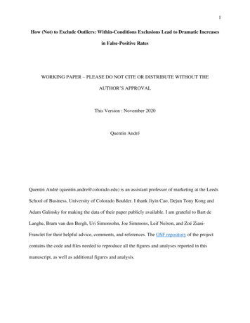
4their data. A boxplot summarizes a distribution by displaying a “box” (representing the 25thpercentile, the median and the 75th percentile of the data) and two “whiskers” (each representinga 1.5 IQR band extending away from the box). Any data point that falls outside of the “whiskers”is flagged as an outlier, with some statistical software (e.g., SPSS) further distinguishing betweenoutliers and “extreme outliers” (further than 3 IQR from the box). Figure 1 displays an examplein the context of an experiment with two conditions: The boxplot identifies no outliers in the“Control” condition, and one outlier in the “Treatment” condition1.Figure 1.From this visualization, a researcher might conclude that it is acceptable (and perhapsdesirable) to identify outliers within conditions. But is this approach correct? In an experimentwith multiple conditions, should one identify and remove outliers across all the data, or withineach condition? Recent papers covering the topic of outlier removal (e.g., Aguinis et al., 2013;Leys et al., 2019) have not broached this important question, and an inspection of the most-cited1This “split-by-condition” boxplot is the default in SPSS, further suggesting that it is the recommendedapproach. To obtain a boxplot across all the data, researchers must instead select the “1-D Boxplot” option.
5books and papers on the topic of univariate outliers (e.g., Barnett & Lewis, 1994; Ghosh & Vogt,2012; Hawkins, 1980; Miller, 1993; Osborne & Overbay, 2004; Ratcliff, 1993) reveals noexplicit discussion of this question2.It is of course not appropriate to apply different exclusion rules to different conditions:One cannot for instance remove all responses that are more than 3 SD away from the mean in the“Control” condition, and all responses that are more than 2 SD away from the mean in the“Treatment” condition. It is transparent that doing so would introduce a systematic differencebetween the two conditions and threaten the researchers’ ability to compare them.But is it appropriate to apply the same exclusion rule (e.g., “any response that is morethan 1.5 IQR lower than the 25th percentile”) within conditions taken separately? For instance,should a researcher, on the basis of the boxplot presented in Figure 1, exclude the “250” responsein the “Treatment” condition, but keep the “250”, “210,” and “200” responses in the “Control”condition? A survey of recent papers published in the Journal of Experimental Psychology:General suggests that it is, indeed, an appropriate decision: Out of 31 papers published in 2019and 2020 that report univariate outliers exclusions, 9 of them are excluding outliers within thedifferent experimental conditions3.In the present article however, I warn that it is in fact not appropriate to identify andexclude outliers within conditions. I highlight that doing so runs against the logic of nullhypothesis significance testing, and present evidence that this practice leads to high false-positiverates, both in simulated and actual data.2To the best of my knowledge, only Cousineau and Chartier (2010) and Meyvis and van Osselaer (2018)have offered an explicit discussion of this question. Both papers (incorrectly) suggest that outliers should be searchedfor, and excluded, within conditions.3A search for all papers including the keyword “outlier” published since 2019 in JEP: General returned 43papers, 31 of which included a univariate exclusion. The spreadsheet summarizing this search is available on theOSF repository of the paper.
6A REFRESHER ON NULL-HYPOTHESIS SIGNIFICANCE TESTINGTo determine if a treatment had an effect, researchers commonly engage in nullhypothesis significance testing (NHST): They compare the observed impact of the treatment towhat would be expected if the treatment did not have any effect (the null hypothesis). This nullhypothesis consists of a set of assumptions about the process that generated the data, and formsthe basis of the statistical set (Nickerson, 2000). For instance, the null hypothesis of a Student ttest is that the two groups were independently sampled at random from a common normaldistribution, and therefore have equal mean.From these assumptions, statisticians derive the theoretical distribution of the teststatistics under the null: The distribution of results that the statistical test would return when thetreatment does not have any effect. The NHST procedure then compares the result observed inthe experiment to this theoretical distribution and returns a p-value: the probability of observing aresult at least as extreme as that of their experiment under the null hypothesis. If the p-value issmaller than a pre-determined threshold (typically α .05), it is common practice to concludethat the null hypothesis is not an appropriate description of the observed data, and to “reject thenull.”However, the p-value thus obtained is only valid if the structure of the data matches theassumptions of the statistical test. When one (or several) assumptions are violated, the theoreticaldistribution of the test statistics under the null (i.e., the distribution of values that is predictedfrom the assumptions of the statistical test) will no longer match the empirical distribution of thetest statistics under the null (i.e., the distribution of values that we will actually observe in the
7experiment when the null hypothesis is true). The test then becomes “inexact,” and itsconclusions may no longer be trusted.Specifically, if extreme values are more frequent in the theoretical distribution than in theempirical distribution, the test is “too conservative”: The threshold to reject the null is too high.On the contrary, if extreme values are less frequent in the theoretical distribution than in theempirical distribution, the test becomes “too liberal”: The threshold to reject the null is too low.EXCLUDING OUTLIERS WITHIN CONDITIONS INVALIDATES NULLHYPOTHESIS TESTINGWhile small deviations from the assumptions are typically inconsequential, largerdeviations can threaten the conclusions of statistical tests. In particular, the practice of excludingoutliers within conditions defies the logic of null-hypothesis significance testing: Whenresearchers choose to exclude outliers within conditions (rather than across the data), they areconsidering that the conditions are different from each other and have therefore implicitlyrejected the null hypothesis. But if we have already accepted that the null hypothesis is not true,how can we then interpret a procedure that assumes that the null is true?This paradox is not simply an intellectual curiosity: When outliers are identified andexcluded within conditions, the data-generating mechanism of the experiment changes, and theassumptions of statistical tests are automatically violated. To illustrate the consequences of thisviolation, consider a simple two-cells experiment first: A team of researchers will elicit a singleresponse from 200 participants, randomly assigned to a “Control” condition or a “Treatment”condition. The researchers are unaware of it, but the treatment does not have any effect: Theresponse for all participants is drawn from the same log-normal distribution.
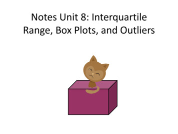
8The researchers will compare the responses in the two conditions using a t-test, but theyare concerned about the presence of outliers. They therefore decide to use a boxplot, and toexclude any participant that is flagged as an outlier prior to analysis. However, the tworesearchers disagree in how the boxplot should be used: Researcher A argues that they shouldidentify and exclude outliers across all the data, while Researcher W believes that they shouldidentify and exclude outliers within each condition. In light of this disagreement, they decide totry both strategies.The histograms in Figure 2 shows the results that each researcher would obtain if theyrepeated the experiment a large number of times. The dashed line on each panel displays thetheoretical null distribution of the t-test: The results that would be expected when theassumptions of the t-test are met (i.e., the two samples are independently sampled at random fromthe same distribution). Since the null hypothesis is correct in this case, we should expect theresults of the experiments to closely match this distribution.
9Figure 2The histogram in the top panel shows the results that Researcher A, who is excludingoutliers across the data, would obtain. We see that these results closely match the theoretical nulldistribution: Extreme differences between conditions are rare, such that the null hypothesis is, asexpected, only rejected 5% of the time. This confirms that excluding outliers across the data doesnot violate the assumptions of the statistical test, and therefore maintains the Type I error at anominal level.In contrast, we see in the bottom panel that the differences observed by Researcher W arelarger than what the theoretical distribution would predict. Differences that the theoretical nulldistribution would consider extremely unlikely are, in fact, relatively common when the outliers
10are excluded within conditions. This translates into a Type I error rate that is grossly inflated:Researcher W would incorrectly reject the null 22% of the time.This result has an intuitive explanation. A key assumption of the null hypothesis of the ttest (and of almost all NHST procedures) is that the samples are drawn from a commondistribution. This assumption is violated once outliers are excluded within conditions: Each of thesamples was submitted to a different data transformation that amplified any pre-existingdifference between them.Figure 3.Figure 3 illustrates this amplification of small differences. The two groups are drawn fromthe same distribution but, by chance, the mean of the “Control” condition is slightly lower than
11the mean of the “Treatment” condition. Because of this minute difference, the same high valuesthat are considered outliers (red dots) in the “Control” condition are not considered as such in the“Treatment” condition. As a consequence, the difference between the two conditions will becomelarger after exclusions. Since the t-test that compares the two conditions does not “know” thatthis procedure was applied to the data, it underestimates the magnitude of the differences that canbe observed under the null, and will reject the null more often than it should. We see that adifference that was originally considered consistent with the null (p .514) becomes a highlysignificant result (p .001) once outliers are excluded within conditions.QUANTIFYING THE PROBLEM IN SIMULATED DATAThis result is not specific to the t-test, or to this particular experiment: When outlierexclusions are not blind to experimental conditions, any statistical procedure that does notaccount for this exclusion procedure will yield invalid conclusions. In support of this claim, Ireport in this section the results of simulated experiments showing that the inflation of falsepositive rates is observed across a variety of statistical tests, data types, sample sizes, andexclusion criteria.I considered 243 (35 ) different experimental setups, obtained by orthogonally crossingthree possible distribution of responses (a normal distribution, a normal distribution withoutliers4, and a log-normal distribution), three possible samples sizes (50, 100 or 250observations per condition), three possible methods (z-score, IQR, and Median AbsoluteDifference) and three possible cutoffs (1.5, 2 or 3 times the z-score/IQR distance/Median4This distribution simulates the presence of large outliers by sampling from a standard normal 𝒩(0, 1) with95% probability or from 𝒩(5, 1) with 5% probability.
12Absolute Difference) for excluding outliers, and three different statistical tests: A parametric testof differences in means (Welsch’s t-test), a non-parametric test of differences in centraltendencies (Mann-Whitney’s U), and a non-parametric test of differences in distribution shapes(the Kolmogorov-Smirnov test)5.To obtain a smooth distribution of the potential outcomes, I generated 10,000 simulatedexperiments in each of those 243 different setups, for a total of 2,430,000 simulated experiments.In each experiment, I draw two samples at random from the same population (such that the nullhypothesis is true), and observe the p-value of the differences between the two samples underthree different outlier exclusion strategies: 1. No exclusions, 2. Exclusions across the data, 3.Exclusions within each condition. For conciseness, I only present the results by exclusion rulesand cutoffs in Figure 4 below. The full breakdown of results (by sample size, data type, statisticaltest, exclusion rules, and exclusion cutoffs) is reported on the OSF repository of the paper.5These three statistical tests cover the majority of the NHST procedures that are applied to continuousunivariate data. For instance, the z-test is the asymptotic equivalent to the t-test when N is large, the F-test of anANOVA is the k-samples analog to the t-test, the Kruskal-Wallis test is the k-samples analog to the Mann-Whitneytest
13Figure 4.Figure 4 presents the survival curves of the tests: The fraction of tests that weresignificant (on the y-axis) at a given significance threshold (on the x-axis), under different outlierexclusion cutoffs (panels) and different outlier exclusion strategies (lines). If the assumptions ofthe statistical procedure are not violated, we should observe nominal false-positives rate: Weshould see that 5% of tests are significant at α .05, that 1% are significant at α .01, and that.1% are significant at α .001. We indeed see this pattern when no outliers are excluded (blue)and when the outliers are excluded across the data (orange), which confirms that those practicesdo not violate the assumptions of the statistical tests.
14In contrast, we observe an increase in false-positive rates when applying the exclusioncutoff within conditions (green line). The simulations show that the increase is systematic andserious, and that it varies significantly across exclusion cutoffs: The most favorable case shows a20% increase in the false-positive rate (from 5% to 6%), and the least favorable case shows a400% increase (from 5% to 20%). In general, we see that the less stringent the cutoff, the moreserious the inflation in false-positive rates: Lower cutoffs increase the number of values excludedwithin each condition, which further amplifies the original differences between the two samples.The full breakdown of results (reported on the OSF repository of the paper) revealssignificant heterogeneity in the severity of the issue across data types and statistical tests. Inparticular, the problem appears to be most severe in the presence of parametric tests (i.e.,Welsch’s t-test) applied to skewed data (i.e., the log-normal distribution), with Type I error ratesalways higher than 10%, and as high as 29%. It is a concerning result: Outliers are mostfrequently excluded in the context of over-dispersed data (e.g., reaction times, willingness-to-pay,sum-scores ), and parametric tests are more commonly used than their non-parametriccounterparts.REPLICATING THE PROBLEM IN RECENT DATAThe conclusions presented so far paint a grim picture: Analysis of simulated data suggestthat excluding outliers will magnify any minute difference between conditions, and lead tounacceptable Type I error rates. In the next section, I demonstrate that the inflation of falsepositive rates is not unique to simulated data, and that the problem is also present (and potentiallymore severe) in actual data collected from human participants. To do so, I propose a re-analysisof a recent paper: Cao, Kong, and Galinsky (2020). This paper offers an interesting case study for
15two reasons: It is one of the most recent paper in a major psychological journal in which outlierswere excluded within conditions, and the authors made the raw data of their paper available.In this paper, the authors report the result of two experiments comparing the negotiationoutcomes (measured by Pareto efficiency) of dyads who were randomly assigned to one of threeconditions: a “No Eating” condition, a “Separate Eating” condition, and a “Shared Eating”condition. The authors find in both experiments that dyads who were assigned to the “SeparateEating” condition have a lower Pareto efficiency than dyads who were assigned to the “SharedEating” condition, and conclude that sharing a meal facilitates cooperation. In both experiments,the outliers are removed within conditions: Any dyad with a Pareto efficiency lower than “threetimes the interquartile range below the lower quartile" of its condition is removed from the data.In addition, it appears that this procedure was recursively applied to the data: After excluding theoutliers, the same threshold is applied again within each condition, and newly identified outliersare removed, until no new outliers are found. This procedure, while unusual, has occasionallybeen recommended to facilitate the identification of outliers in heterogeneous data (Meyvis &Van Osselaer, 2018; Schwertman & de Silva, 2007; Van Selst & Jolicoeur, 1994).
16Figure 5/Having access to the authors’ raw data allows me to compare the results obtained in eachstudy under different exclusion strategies (Figure 5). The upper-left panel presents the authors’original results: When outliers are iteratively excluded within conditions, the difference betweenthe “Separate Eating” and the “Shared Eating” condition is large and significant. However, wesee that this difference is attenuated when only round of exclusion is performed within conditions(upper-left panel), and shrinks to a small, non-significant amount when outliers are excludedacross conditions (bottom-left panel) or when no exclusions are performed (bottom-right panel).This descriptive analysis confirms that excluding outliers within conditions can magnify smalldifferences that are originally present between conditions.
17This analysis does not necessarily mean that the authors’ result is a false-positive (toreach this conclusion, one would need to know whether the null hypothesis is true). However,one can compute the likelihood of observing a false-positive in the context of the authors’experiment. To do so, I reassign the condition labels in the data of Study 2 at random6 (so that thedifferences between conditions are truly zero in expectation), perform a t-test on the two groups,and check how often the Pareto efficiency of dyads in the “Separate Eating” is significantlydifferent from the Pareto efficiency of dyads in the “Shared Eating” condition.6I focus on Study 2 because it was pre-registered, but similar results (reported on the OSF repository of thepaper) are observed in Study 1.
18Figure 6.Figure 6 replicates the Type I error inflation previously observed in simulated data (theexclusion criteria used by the authors, removing observations that are at least three times theinterquartile range below the lower quartile, appears in the upper right corner). While outlierexclusions are not associated with higher false-positive rates when they are performed across thedata (the orange line), the likelihood of a false-positive result increases sharply when outliers areexcluded within conditions (the green line): It is always higher than 10%, and can be as high as47%.Finally, this figure shows that the increase is even stronger when the outliers areiteratively excluded within conditions (the red line). This result is not surprising: Iteratedexclusions are causing the two conditions to diverge even further, and routinely lead todifferences that the theoretical null distribution would consider extremely unlikely. In particular,the upper right panel show that the exclusion strategy and cutoff reported in the paper isassociated with a false-positive rate of 56%, which translates into a false-positive rate of 28% forthe directional hypothesis pre-registered by the authors.SUMMARY AND RECOMMENDATIONSA survey of the recent literature, and the common practice of splitting boxplots byconditions, suggest that excluding outliers within conditions is an acceptable strategy. I havedemonstrated that this conclusion is erroneous: Excluding outliers by condition amplifies thesmall differences that are normally expected under the null, which results in inflated Type I errorrates. This result is observed for parametric and non-parametric tests, different exclusion criteria,different cutoffs, different sample sizes, and in both simulated and real data. In light of these
19results, I conclude that the practice of excluding outliers within conditions is a “questionableresearch practice” that makes false-positive far too likely (Simmons et al., 2011), and that itshould be abandoned by researchers.What if the Pattern of Responses Does Differ Across Conditions?It might be tempting to justify the practice of excluding outliers within conditions by theobservation that the conditions look different: One condition appears to have a higher mean, or asmaller dispersion, than the other(s). As mentioned earlier however, this justification is aparadox: If we assume that the pattern of responses differ across conditions, we have alreadyrejected the null hypothesis, which then begs the interest of using a statistical test to comparethem. If the researchers know that the values differ across conditions (e.g., when measuring theheight of adults vs. children, or how testing how fast people can solve an easy vs. hard mathpuzzle), then they do not need a statistical test to compare the conditions, and can excludeoutliers by group. However, if they want to test for the presence of a difference between theconditions, they cannot exclude outliers by condition and apply a regular statistical test.Can Researchers Ignore this Problem if they Apply a Stricter Alpha Level, or if they UseBayesian Statistics?Using a stricter alpha level would not solve the issue. First, the exact impact of excludingoutliers within conditions on false-positive rates is variable and unpredictable: In the simulationsand in real data, the increase could be as low as 20% (from 5% to 6%), and as high as 940%(from 5% to 47%), depending on the type of statistical test, the rule for excluding outliers, andthe exact structure of the data. As a consequence, it is unclear how large of a correctionresearchers should apply. Second, the stricter the alpha level, the lower the power of the test (all
20other things being equal): Researchers should not adopt a practice that would harm their ability todetect true effects when better alternatives are available.The default estimation procedures in the Bayesian researcher toolbox (e.g., the Bayesiant-test; Kruschke, 2013) would also not offer a remedy. Indeed, the problem is not specific toNHST, and Bayesian inferences also hinges on the assumption that the data-generatingmechanism is correctly identified (Gelman et al., 2013). For this reason, any procedure that doesnot explicitly model the per-condition exclusion (and therefore does not account for the inflationof differences between conditions) will also yield inaccurate results. In support of this claim, Ipresent additional analysis (reported on the OSF repository of the paper) showing that when aBayesian t-test is applied to null data, the highest density interval (HDI, the Bayesian counterpartof the confidence interval) contains zero more frequently when exclusions are performed withincondition exclusions (vs. across the data).How Should Researchers Deal with Outliers Then?The simplest recommendation would be to exclude outliers across the data, and not withinconditions. As shown in the simulations presented in this article, this practice does not cause aType I error inflation.A second possibility would be not to exclude the outliers, and to analyze the data usingnon-parametric tests (e.g., rank-based tests, or resampling-based tests; Erceg-Hurn & Mirosevich,2008), or heavy-tailed Bayesian models (e.g., West, 1984), that are less sensitive to the presenceof extreme values.Finally, if sample sizes are small, and if power to detect an effect is an important concern,researchers may consider using specific estimators developed for trimmed and winsorized groups(e.g., Kim, 1992; Wilcox, 2011; Wu, 2006; Yuen, 1974). These specific procedures account for
21the fact that the data was transformed within conditions, and therefore maintain a nominal Type Ierror rate. However, they come at some overhead to the researcher: It is important to select theestimator that matches the exclusion strategy that was used (i.e., deviation from mean or median;removing vs. winsorizing), and the design of the experiment (between-subjects, within-subjects,or mixed design).What If the Experiment Design is More Complex?The present paper discussed the problem of by-condition exclusions in the context ofsingle-factor experiments. However, the same general principle applies to make complex designs(e.g., factorial, or repeated-measure designs): Any outlier exclusion procedure must be blind tothe factor(s) that researchers are interested in testing. The following examples illustrate this rule.Example 1: A between-subject factorial design in which participants are randomlyassigned to solve one easy (vs. hard) math puzzle after engaging in a mindfulness (vs. relaxation)workshop.It is clear that people will take more time to solve the hard math puzzle than the easy mathpuzzle. Researchers can therefore choose not to test for the impact of puzzle difficulty, and toexclude outliers within the “hard puzzle” and “easy puzzle” conditions taken separately.However, they cannot exclude outliers within the “mindfulness” and the “relaxation” conditionstak
outliers and “extreme outliers” (further than 3 IQR from the box). Figure 1 displays an example in the context of an experiment with two conditions: The boxplot identifies no outliers in the “Control” condition,