WIXLIB

MODULEIdentifying andAddressing Outliers5 DATA FILES FOR THIS MODULEmodule5 jobsatis.savmodule5 jobsatis final.sav KEY LEARNING OBJECTIVESThe student will learn to use summary descriptive statistics (e.g., skewness and kurtosis) to helpdetermine the shape of a continuous variable’s distribution create and interpret stem-and-leaf plots and boxplots to help determinethe shape of a distribution and identify outliers create, interpret, and compare a set of boxplots for a continuous variableby groups of a categorical variable conduct and compare t-tests on data with outliers and data without outliers to determine whether the outliers have an impact on results.A. Description of Researcher’s Study This module is a continuation of Dr. Mendoza’s collaboration with a company that is conducting experimental research to improve the level of jobsatisfaction among its employees. In Module 4, he examined the distributions for descriptive variables in his current data file as well as scores on anassessment of knowledge and aptitude. Using frequency tables, crosstabs,and histograms to display information about the distributions, he mademodifications to condense the number of groups for the nominal andordinal variables and to change the measurement scale of one variable fromratio (continuous) to ordinal (categorical).– 81

82–– THE NATURE AND DISTRIBUTION OF VARIABLESHere, Dr. Mendoza will examine the final two continuous variables inthe data file, which contain scores on two instruments designed to measuremotivation and job satisfaction prior to the beginning of the 3-month study.This module demonstrates how he used boxplots to look at the shape of thedistributions, identify potential outliers, and decide how outliers will behandled when analyzing the data. Upon completion of the study, the instruments will be administered again to measure potential change in the constructs for employees who received the job enrichment program and tocompare results to those who did not receive the program.B. A Look at the DataThe data file used in this module (module5 jobsatis.sav) contains all nineoriginal variables in Dr. Mendoza’s initial file plus the newly modified variables he created in Module 4. There are 265 cases (participants) and a totalof 12 variables. As before, each case represents one employee who agreedto be in the study. Employees are in one of seven geographic locations of thecompany. A total of 127 participants are receiving the job enrichment program, and the remaining 138 participants are in the control group. Table 5.1lists each variable and its description.Table 5.1  Variables in the Job Satisfaction Data FileVariable Name Descriptionidnumerical identifier for each participant 1 to 265locationgeographic location of the company in which the participantis employed, coded 1 to 7program0 no (participant is not receiving the program, he or she isin the control group); 1 yes (participant is receiving theprogram)sizetotal number of employees in each geographic location of thecompany across all its sectors. This variable is a constant valuefor participants within the same location.yrs expertotal number of years of experience within the company foreach participant. Codes for the categories are 2 0 to 2 yearsof experience, 4 3 to 4 years of experience, 6 5 to 6 yearsof experience, 8 7 to 8 years of experience, 10 9 to 10years of experience, and so on until the final code of 32 31years of experience or more.

Identifying and Addressing Outliers–– 83Variable Name Descriptionreprimandtotal number of reprimands received by each employeeduring his or her total years of experience with the companyaptitudescore on an aptitude instrument prior to implementingthe studymotivationscore on a motivation survey prior to implementing the studyjob satisscore on a job satisfaction survey prior to implementingthe studylocation rrevised variable with only five codes (1, 3, 6, 7, and 9). Due tothe small number of participants in locations 2, 4, and 5, theselocations were combined and assigned a new code of 9.yrs exper rrevised variable with only six codes (2, 4, 6, 8, 10, and 30).The first original five codes remained unchanged. Due tosmall sample sizes in the remaining codes, they werecombined into a new code of 30 that represents participantswith 11 or more years of experience.reprimand rrevised variable is now an ordinal variable with three levels: 0reprimands, 1 reprimand, and 2 or more reprimands. Originalvalues of 2, 3, and beyond were collapsed into one level dueto small sample sizes.C. Planning and Decision MakingTo examine prescores on the two constructs of motivation and job satisfaction, Dr. Mendoza decided to create boxplots in SPSS. There are severalbeneficial features of this type of graphic display. First, it allows you to viewaspects of the distribution in a way that histograms do not. The length of the“box” spans the middle 50% of the values, that is, from the 1st quartile(25th percentile) to the 3rd quartile (75th percentile), and the medianappears as a solid line in the box. In a distribution with no outliers, thelength of the two “whiskers” represent the bottom 25% of values and thetop 25% of values. When a distribution is approximately normal, the medianwill be in the center of the “box” and the two “whiskers” will be equal inlength. The extent to which this does not occur indicates potential positiveor negative skewness or kurtosis.A second beneficial feature of the boxplot over the histogram is thatit can identify potential outliers. Outliers are values at the lower or

84–– THE NATURE AND DISTRIBUTION OF VARIABLESupper end that lie apart from the distribution. These values are identified onthe box plot as cases below or above theend of each “whisker.” More specifically, SPSS identifies outliers as casesthat fall more than 1.5 box lengths fromthe lower or upper hinge of the box.The box length is sometimes called the“hspread” and is defined as the distancefrom one hinge of the box to the otherhinge. It is also called the interquartilerange. SPSS further distinguishes“extreme” outliers by identifying valuesmore than 3 box lengths from eitherhinge. **Dr. Mendoza (1)Statistical inferential tests can be quite sensitive to outliers, oftenbecause the calculations rely on squared deviations from the mean. Oneor two values that are far from the mean can alter the results considerably.Therefore, if outliers are identified, Dr. Mendoza must decide how tohandle them. First, he will go back to the data collection instrumentationto determine whether the outlier was due to a data entry error or aninstrumentation error. The former can be corrected, and the latter probably should be deleted. However, if the outlier was not due to one ofthese reasons and was an actual value obtained from the participant, thenhe has a few options. The most undesirable option is to delete the casefrom further analysis. This is not the best solution because the value is alegitimate case in the data file, and with large samples, it can be expectedthat a few outliers may occur and probably will not greatly impact results.Another option is to conduct data analysis with and without the outlier(s)and compare the two outcomes. If results are the same, then theoutlier(s) did not have a great influence in the distribution of the variable.If results are not the same, both outcomes can be reported. A thirdoption is to transform the variable and hopefully reduce the influence ofthe outlier(s). Finally, outliers could be recoded into the lowest (or highest) value that is not determined to be an outlier by SPSS (or any othermethod that is used).Dr. Mendoza will obtain the boxplots for motivation and job satis usingthe Explore procedure. Although there are a few other ways to get boxplots in SPSS, he chose this procedure because it produces descriptive statistics such as skewness and kurtosis as well as a stem-and-leaf plot, which isanother type of visual display of data.**1 Dr. Mendoza says: “There is not ahard and fast rule for identifying outliers in a distribution. SPSS uses oneparticular method, but others exist. Forexample, standardized values can beused with a general guideline thatabsolute z values larger than 3 areconsidered to be outliers. However, forlarge samples, some statisticians use acutoff z value of 4 or greater, and forsmall sample sizes, a cutoff of 2.5”(Stevens, 2009).

Identifying and Addressing Outliers–– 85D. Using SPSS to Address Issues and Prepare DataMotivationA visual scroll through the data file is sometimes the first indication aresearcher has that potential outliers may exist. For motivation, Dr. Mendozanoticed that a few low scores seemed to stand apart from the rest of the distribution. To help him determine whether these low values are actually outliers, he obtained a boxplot under the Analyze menu. Selecting DescriptiveStatistics and Explore produced the dialog box shown in Figure 5.1. Heplaced motivation in the Dependent List box.Figure 5.1   Analyze Descriptive Statistics ExploreDr. Mendoza kept the default settings under the Statistics and Plotsbuttons as is. The Options button offers different ways to treat missingvalues, but he has none in his study, so he does not need the options. Asshown in Figure 5.2, the default for Statistics is Descriptives. This willproduce a variety of descriptive summary statistics for motivation, includingthe skewness and kurtosis values.

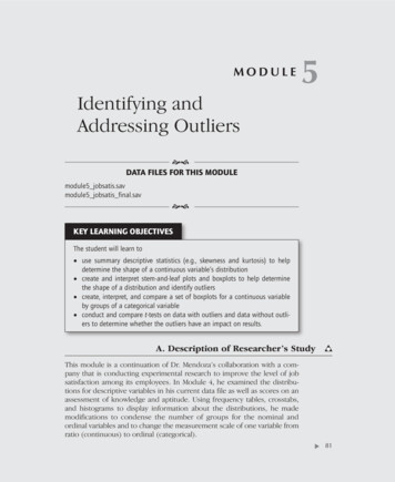
86–– THE NATURE AND DISTRIBUTION OF VARIABLESFigure 5.2   Statistics in ExploreFor Plots, the default is to produce a boxplot and a stem-and-leaf plot,as shown in Figure 5.3.Figure 5.3   Plots in ExploreAfter he clicked OK in the Explore dialog box, Dr. Mendoza obtainedoutput that includes a table of values, a stem-and-leaf plot, and a boxplot.Table 5.2 displays the summary descriptive statistics. He noticed that themean, median, and trimmed mean are nearly identical. This is one indication

Identifying and Addressing Outliers–– 87that the distribution is not skewed in oneSPSS Tip 1: A distribution with a condirection or another. To examine skewnesssiderably high positive kurtosis value isand kurtosis, Dr. Mendoza used the stancalled leptokurtic, meaning that it isdard errors provided for each value inslender and narrow. A distribution withorder to obtain standardized values fora considerably high negative kurtosiseach statistic. Dividing skewness by thevalue is called platykurtic, meaningstandard error (–.602 divided by .150)flat or broad. Low absolute valuesyields a standardized value of –4.01, whichclose to 0 for kurtosis are said to bedoes indicate a somewhat negativelymesokurtic or intermediate.skewed distribution. In a similar fashion,he divided kurtosis by its standard error(1.891 divided by .298) to obtain a standardized value of 6.35, which indicates a peaked, or slender and narrow,distribution. **SPSS Tip 1 Dr. Mendoza kept these values in mind as helooked at the next section of output from the Explore procedure.Table 5.2   First Portion of SPSS Explore Output: Summary Statistics for MotivationDescriptivesStatisticMotivationMeanStd. Error20.0295% Confidence Interval forLower Bound19.58MeanUpper Bound20.455% Trimmed Mean20.11Median20.00Variance12.932Std. e Range.2214Skewness-.602.150Kurtosis1.891.298Figure 5.4 displays the stem-and-leaf plot. The stems represent the twodigit data values for motivation. Each leaf represents a case with that particular data value. The frequency column represents the total number of cases