Transcription
Lectures on Algebraic TopologyLectures by Haynes MillerNotes based in part on a liveTEXed record made by Sanath DevalapurkarAugust 27, 2021i
iiTo Juli
iiiPrefaceAlgebraic topology is a fundamental and unifying discipline. It was the birthplace of many ideaspervading mathematics today, and its methods are ever more widely utilized.These notes record lectures in year-long graduate course at MIT, as presented in 2016–2017.The second semester was given again in the spring of 2020. My goal was to give a pretty standardclassical approach to this subject, but with an eye to more recent perspectives. I wanted to introducestudents to the basic language of category theory, homological algebra, and simplicial sets, so usefulthroughout mathematics and finding their first real manifestations in algebraic topology. On theother hand I barely touched on some important subjects. I did not talk about simplicial complexesat all, nor about the Lefschetz fixed point theorem. I gave only a brief summary of the theory ofcovering spaces and the fundamental group, which are regarded as prerequisites for this course.In the first part, I especially wanted to give an honest account of the machinery – relative capproduct and Čech cohomology – needed in the proof of Poincaré duality. The present documentcontains a bit more detail on these matters than was presented in the course itself. The 2020 coursewas disrupted by the COVID-19 pandemic, and the entire simplicial development of classifyingspaces, Lectures 57–59, were consequently omitted. The pace picked up speed as the course wentalong, and we ended with a cursory treatment of Thom’s work on cobordism. In this second half, Iprobably didn’t cover quite as much in the lectures as is written in this text.This is a volume of lecture notes, not a textbook! (There are good ones: [72, 69, 10, 15, 24, 36, 50]for example.) I have been inspired by the admirable examples set by the authors of [14] and [59]. Ihave opted for variety rather than completeness. Most lectures conclude with a series of exercises,most of which were actually assigned as part of the course. They vary widely in difficulty.I was lucky enough to have in the audience a student, Sanath Devalapurkar, who spontaneouslydecided to liveTEX the entire course. This resulted in a remarkably accurate record of what happenedin the classroom – right down to random alarms ringing and embarrassing jokes and mistakes on theblackboard. Sanath’s TEX forms the basis of these notes, and I am grateful to him for making themavailable. The attractive drawings in the first half were provided by another student, XianglongNi, who also carefully proofread the manuscript. Chapters 4–8 reflect the 2020 class and so departmore from the original notes.In addition to Sanath and Xianglong, I am delighted to thank the generations of studentswho have kept me on track and honest over several decades of teaching this subject. I owe aparticular debt to Phil Hirschhorn, Stefan Jackowski, Calder Morton-Ferguson Timothy Ngotiaoco,and Manuel Rivera, each of whom pointed out errors in the text and suggested corrections. Ofcourse many inaccuracies are guaranteed to remain, a reality for which I apologize.Newton, MADecember, 2020
ContentsContentsiv1 Singular homology1Introduction: singular simplices and chains . . . . .2Homology . . . . . . . . . . . . . . . . . . . . . . . .3Categories, functors, and natural transformations . .4Categorical language . . . . . . . . . . . . . . . . . .5Homotopy, star-shaped regions . . . . . . . . . . . .6Homotopy invariance of homology . . . . . . . . . . .7Homology cross product . . . . . . . . . . . . . . . .8Relative homology . . . . . . . . . . . . . . . . . . .9Homology long exact sequence . . . . . . . . . . . . .10 Excision and applications . . . . . . . . . . . . . . .11 Eilenberg-Steenrod axioms and the locality principle12 Subdivision . . . . . . . . . . . . . . . . . . . . . . .13 Proof of the locality principle . . . . . . . . . . . . .2 Computational methods14 CW complexes I . . . . . . . . . . . . . . . . . .15 CW complexes II . . . . . . . . . . . . . . . . . .16 Homology of CW complexes . . . . . . . . . . . .17 Real projective space . . . . . . . . . . . . . . . .18 Euler characteristic and homology approximation19 Coefficients . . . . . . . . . . . . . . . . . . . . .20 Tensor product . . . . . . . . . . . . . . . . . . .21 Tensor and Tor . . . . . . . . . . . . . . . . . . .22 Fundamental theorem of homological algebra . .23 Hom and Lim . . . . . . . . . . . . . . . . . . . .24 Universal coefficient theorem . . . . . . . . . . .25 Künneth and Eilenberg-Zilber . . . . . . . . . . .3 Cohomology and duality26 Coproducts, cohomology . . . . . . . .27 Ext and UCT . . . . . . . . . . . . . .28 Products in cohomology . . . . . . . .29 Cup product, continued . . . . . . . .30 Surfaces and nondegenerate symmetric31 Local coefficients and orientations . . . . . . . . . . . . . . . . . . . . . . . . . . . . . . .bilinear forms. . . . . . . 77174.79798386889195
CONTENTS32333435363738Proof of the orientation theorem . . . . .A plethora of products . . . . . . . . . . .Cap product and Čech cohomology . . . .Čech cohomology as a cohomology theoryFully relative cap product . . . . . . . . .Poincaré duality . . . . . . . . . . . . . .Applications . . . . . . . . . . . . . . . . .v.1011041061101131161194 Basic homotopy theory39 Limits, colimits, and adjunctions . . . . . . . . . . .40 Cartesian closure and compactly generated spaces . .41 Basepoints and the homotopy category . . . . . . . .42 Fiber bundles . . . . . . . . . . . . . . . . . . . . . .43 Fibrations, fundamental groupoid . . . . . . . . . . .44 Cofibrations . . . . . . . . . . . . . . . . . . . . . . .45 Cofibration sequences and co-exactness . . . . . . . .46 Weak equivalences and Whitehead’s theorems . . . .47 Homotopy long exact sequence and homotopy fibers.1231231271311341361411441471515 topy theory of CW complexesSerre fibrations and relative lifting . . . . . . .Connectivity and approximation . . . . . . . .The Postnikov tower . . . . . . . . . . . . . . .Hurewicz, Eilenberg, Mac Lane, and WhiteheadRepresentability of cohomology . . . . . . . . .Obstruction theory . . . . . . . . . . . . . . . .6 Vector bundles and principal bundles54 Vector bundles . . . . . . . . . . . . . . . . . .55 Principal bundles, associated bundles . . . . . .56 G-CW complexes and the I-invariance of BunG57 The classifying space of a group . . . . . . . . .58 Simplicial sets and classifying spaces . . . . . .59 The Čech category and classifying maps . . . .7 Spectral sequences and Serre classes60 Why spectral sequences? . . . . . . . . . . . . . . . . . .61 Spectral sequence of a filtered complex . . . . . . . . . .62 Serre spectral sequence . . . . . . . . . . . . . . . . . . .63 Exact couples . . . . . . . . . . . . . . . . . . . . . . . .64 Gysin sequence, edge homomorphisms, and transgression65 Serre exact sequence and the Hurewicz theorem . . . . .66 Double complexes and the Dress spectral sequence . . .67 Cohomological spectral sequences . . . . . . . . . . . . .68 Serre classes . . . . . . . . . . . . . . . . . . . . . . . . .69 Mod C Hurewicz and Whitehead theorems . . . . . . . .70 Freudenthal, James, and Bousfield . . . . . . . . . . . .
vi8 Characteristic classes, Steenrod operations, and cobordism71 Chern classes, Stiefel-Whitney classes, and the Leray-Hirsch theorem72 H (BU (n)) and the splitting principle . . . . . . . . . . . . . . . . .73 Thom class and Whitney sum formula . . . . . . . . . . . . . . . . .74 Closing the Chern circle, and Pontryagin classes . . . . . . . . . . . .75 Steenrod operations . . . . . . . . . . . . . . . . . . . . . . . . . . .76 Cobordism . . . . . . . . . . . . . . . . . . . . . . . . . . . . . . . . .77 Hopf algebras . . . . . . . . . . . . . . . . . . . . . . . . . . . . . . .78 Applications of cobordism . . . . . . . . . . . . . . . . . . . . . . . 93Index297
Chapter 1Singular homology1Introduction: singular simplices and chainsThis is a course on algebraic topology. The objects of study are of course topological spaces, andthe machinery we develop in this course is designed to be applicable to a general space. But we arereally mainly interested in geometrically important spaces. Here are some examples. The most basic example is n-dimensional Euclidean space, Rn . The n-sphere S n {x Rn 1 : x 1}, topologized as a subspace of Rn 1 . Identifying antipodal points in S n gives real projective space RPn S n /(x x), i.e. thespace of lines through the origin in Rn 1 . Call an ordered collection of k orthonormal vectors in a real inner product space an orthonormal k-frame. The space of orthonormal k-frames in Rn , topologized as a subspace of (S n 1 )k ,forms the Stiefel manifold Vk (Rn ). For example, V1 (Rn ) S n 1 . The Grassmannian Grk (Rn ) is the space of k-dimensional linear subspaces of Rn . Formingthe span gives us a surjection Vk (Rn ) Grk (Rn ), and the Grassmannian is given the quotienttopology. For example, Gr1 (Rn ) RPn 1 .All these examples are manifolds; that is, they are Hausdorff spaces locally homeomorphic to Euclidean space. Aside from Rn itself, they are also compact. Such spaces exhibit a hidden symmetry,which is the culmination of the first half of this course: Poincaré duality.Simplices and chainsAs the name suggests, the central aim of algebraic topology is the usage of algebraic tools to studytopological spaces. A common technique is to probe topological spaces via maps to them fromsimpler spaces. In different ways, this approach gives rise to singular homology and homotopygroups. We now detail the former; the latter takes the stage in the second half.Definition 1.1. For n 0, the standard n-simplex n is the convex hull of the standard basis{e0 , . . . , en } in Rn 1 :nXoX n ti ei :ti 1, ti 0 Rn 1 .Each ei is a vertex of the simplex (plural “vertices”). The ti are called barycentric coordinates.1
2CHAPTER 1. SINGULAR HOMOLOGYThe word “simplex” comes from the Latin, and should suggest “simple” in the sense of “notcompound.” In mathematics its plural is always “simplices.” There is a well-developed theoryof simplicial complexes, appropriately organized unions of simplices, which however we will notdevelop in these lectures. Here the word “complex” is used, as it is in “complex number,” not todenote complexity but rather “compound” (of real and imaginary parts, in the case of numbers).The standard simplices are related by face inclusions di : n 1 n for 0 i n, where di isthe affine map that sends vertices to vertices, in order, and omits the vertex ei .11121001001Definition 1.2. Let X be any topological space. A singular n-simplex in X is a continuous mapσ : n X. We will often drop the adjective “singular.” Denote by Sinn (X) the set of alln-simplices in X.This seems like a rather bold construction to make, as Sinn (X) is huge. But be patient! Forthe moment, notice the peculiar use of the word “singular.” It derives from the notion that theimage of the map σ might have cusps or kinks or other kinds of “singularities” – another specializedmathematical term, indicating that these points are unusual and special.For 0 i n, precomposition by the face inclusion di produces a map di : Sinn (X) Sinn 1 (X)sending σ to σ di . This is the “ith face” of σ. This allows us to make sense of the “boundary” of asimplex.For example, if σ is a 1-simplex that forms a closed loop, then d1 σ d0 σ. We would liketo re-express this equality as a statement that the boundary “vanishes” – we would like to write“d0 σ d1 σ 0.” Here we don’t mean to subtract one point of X from another! Rather we meanto form a “formal difference.” To accommodate such formal sums and differences, we will enlargeSinn (X) still further by forming the free abelian group it generates.Definition 1.3. The abelian group Sn (X) of singular n-chains in X is the free abelian groupgenerated by n-simplices,Sn (X) ZSinn (X) .So an n-chain is a finite linear combination of n-simplices,kXai σi ,ai Z ,σi Sinn (X) .i 1If n 0, Sinn (X) is declared to be empty, so Sn (X) 0.We can now define the boundary operatord : Sinn (X) Sn 1 (X) ,
1. INTRODUCTION: SINGULAR SIMPLICES AND CHAINS3bydσ nX( 1)i di σ .i 0This extends to a homomorphism d : Sn (X) Sn 1 (X) by additivity.We use this homomorphism to obtain something more tractable than the entirety of Sn (X).First we restrict our attention to chains with vanishing boundary.Definition 1.4. An n-cycle in X is an n-chain c with dc 0. An n-chain is a boundary if it is inthe image of d : Sn 1 (X) Sn (X). Notation:Zn (X) ker(d : Sn (X) Sn 1 (X)) ,Bn (X) im(d : Sn 1 (X) Sn (X)) .For example, a 1-simplex is a cycle if its ends coincide. More generally, a sum of 1-simplices isa cycle if the right endpoints match up with the left endpoints. Geometrically, you get a collectionof loops, or “cycles.” This is the origin of the term “cycle.”Every 0-chain is a cycle, since S 1 (X) 0.Singular homologyIt turns out that there’s a cheap way to produce cycles:Theorem 1.5. Any boundary is a cycle; that is, d2 0.We’ll leave the verification of this important result as a homework problem. What we havefound, then, is that the singular chains form a “chain complex,” as in the following definition.Definition 1.6. A graded abelian group is a sequence of abelian groups, indexed by the integers. Achain complex is a graded abelian group {An } together with homomorphisms d : An An 1 withthe property that d2 0.We have just defined the singular chain complex S (X) of a space X.The chains that are cycles by virtue of being boundaries are the “cheap” ones. If we quotient bythem, what’s left is the “interesting cycles,” captured in the following definition.Definition 1.7. The nth singular homology group of X is:Hn (X) ker(d : Sn (X) Sn 1 (X))Zn (X) .Bn (X)im(d : Sn 1 (X) Sn (X))We use the same language for any chain complex: it has cycles, boundaries, and homologygroups. The homology forms a graded abelian group. Two cycles that differ by a boundary are saidto be homologous. (The word “homology” arose first in biology to indicate a shared evolutionaryorigin.)Both Zn (X) and Bn (X) are free abelian groups because they are subgroups of the free abeliangroup Sn (X), but the quotient Hn (X) isn’t necessarily free. While Zn (X) and Bn (X) are uncountably generated, Hn (X) turns out to be finitely generated for the spaces we are interested in! If T isthe torus, for example, then we will see that H1 (T ) Z Z, with generators given by the 1-cyclesillustrated below.
4CHAPTER 1. SINGULAR HOMOLOGYWe will learn to compute the homology groups of a wide variety of spaces. The n-sphere forexample has the following homology groups: Zif q n 0 Zif q 0, n 0Hq (S n ) Z Z if q n 0 0otherwise .There is an interesting n-cycle, that, roughly speaking, covers every point of the sphere exactly once.Any q-cycle with q different from 0 and n is a boundary, so it doesn’t contribute to the homology.ExercisesExercise 1.8. (a) Let [n] denote the totally ordered set {0, 1, . . . , n}. Let φ : [m] [n] be anorder preserving function (so that if i j then φ(i) φ(j)). Identifying the elements of [n]with the vertices of the standard simplex n , φ extends to an affine map m n that wealso denote by φ. Give a formula for this map in terms of barycentric coordinates: If we writeφ(s0 , . . . , sm ) (t0 , . . . , tn ), what is tj as a function of (s0 , . . . , sm )?(b) Write dj : [n 1] [n] for the order preserving injection that omits j as a value. Show thatan order preserving injection φ : [n k] [n] is uniquely a composition of the form djk djk 1 · · · dj1 ,with 0 j1 j2 · · · jk n. Do this by describing the integers j1 , . . . , jk directly in terms ofφ, and then verify the straightening ruledi dj dj 1 difor i j .(c) Show that any order preserving map φ : [m] [n] factors uniquely as the composition of anorder preserving surjection followed by an order preserving injection.(d) Write si : [m 1] [m] for the order-preserving surjection that repeats the value i. Show thatany order-preserving surjection φ : [m] [n] has a unique expression si1 si2 · · · sik with n i1 i2 · · · ik 0. Do this by describing the numbers i1 , . . . , ik , directly in terms of φ, and finding astraightening rule of the form si sj · · · for i j.(e) Finally, implement your assertion that any order preserving map factors as a surjection followedby an injection by establishing a straightening rule of the form si dj · · · .Recall the notation Sinn (X) for the set of continuous maps from n to the space X. The affineextension φ : m n of an order-preserving map φ : [m] [m] induces a map φ : Sinn (X) Sinm (X). In particular, writedi (di ) sj (sj ) .The di ’s are face maps, the si ’s are degeneracies.(f ) Write down the identities satisfied by these operators, resulting from the identities you foundrelating the di ’s and sj ’s.
2. HOMOLOGY5A simplicial set is a sequence of sets K0 , K1 , . . ., with maps di : Kn Kn 1 , 0 i n, andsi : Kn Kn 1 , 0 i n, satisfying these identities. The elements of Kn are the “n-simplices”of K; when n 0 they are the “vertices” of K. For example, we have the singular simplicial setSin (X) of a space X.(g) Use the relations among the di ’s to prove thatd2 0 : Sn (X) Sn 2 (X) .2HomologyIn the last lecture we introduced the standard n-simplex n Rn 1 . Singular simplices in a spaceX are maps σ : n X and constitute the set Sinn (X). For example, Sin0 (X) consists of pointsof X. We also described the face inclusions di : n 1 n , and the induced “face maps”di : Sinn (X) Sinn 1 (X) ,0 i n,given by precomposing with face inclusions: di σ σ di . For homework you established somequadratic relations satisfied by these maps. A collection of sets Kn , n 0, together with mapsdi : Kn Kn 1 related to each other in this way, is a semi-simplicial set. So we have assigned to anyspace X a semi-simplicial set S (X). (You actually get a simplicial set; but, while the “degeneracies”will ultimately play an important role, they do not enter into the definition of singular homology.Simplicial sets were originally called “complete semi-simplicial complexes”; “semi-simplicial” becausethey weren’t necessarily simplicial complexes, and “complete” because they included degeneracies.Current usage recycles the “semi-” to mean that only the face maps are used, not the degeneracies.)To the semi-simplicial set {Sinn (X), di } we then applied the free abelian group functor, obtaininga semi-simplicial abelian group. Forming alternating sums of the di s, we constructed a boundarymap d which makes S (X) a chain complex – that is, d2 0. We capture this process in a diagram:{spaces}H / {graded abelian groups}OSin {semi-simplicial sets} homologyZ( ){semi-simplicial abelian groups}/ {chain complexes}Example 2.1. Suppose we have σ : 1 X. Define φ : 1 1 by sending (t, 1 t) to (1 t, t).Precomposing σ with φ gives another singular simplex σ which reverses the orientation of σ. It isnot true that σ σ in S1 (X).However, we claim that σ σ mod B1 (X). This means that there is a 2-chain in X whoseboundary is σ σ. If d0 σ d1 σ, so that σ Z1 (X), then σ and σ are homologous cycles, so that[σ] [σ] in H1 (X).To construct an appropriate “homology” – a 2-chain τ with the property that dτ σ σ –consider the projection map π : 2 1 that is the affine extension of the map sending e0 and e2to e0 and e1 to e1 . (Incidentally this is not a degeneracy since it is not order-preserving.)
6CHAPTER 1. SINGULAR HOMOLOGY21100We’ll compute d(σ π). Some of the terms will be constant singular simplices. Let’s writecnx : n Xfor the constant map with value x X. Thend(σ π) σπd0 σπd1 σπd2 σ c1σ(0) σ .The constant simplex c1σ(0) is an “error term,” and we wish to eliminate it. To achieve this we canuse the constant 2-simplex c2σ(0) at σ(0); its boundary isc1σ(0) c1σ(0) c1σ(0) c1σ(0) .Soσ σ d(σ π c2σ(0) ) ,and σ σ mod B1 (X) as claimed.Let’s compute the singular homology of the very simplest spaces, and . For the first,Sinn ( ) , so Sn ( ) 0. Hence S ( ) is the zero chain complex. This means that Z ( ) B ( ) 0. The homology in all dimensions is therefore 0.For , we have Sinn ( ) {cn } for all n 0. Consequently Sn ( ) Z for n 0 and 0 for n 0.Suppose n 0. For each i, di cn cn 1, so the boundary maps d : Sn ( ) Sn 1 ( ) in the chain complex depend on the parity of n as follows:(nXcn 1for n even, and ni n 1d(c ) ( 1) c 0for n odd.i 0This means that our chain complex is:01010 Z Z Z Z ··· .The boundaries coincide with the cycles except in dimension zero, where B0 ( ) 0 while Z0 ( ) Z.Therefore H0 ( ) Z and Hi ( ) 0 for i 6 0.Induced mapsWe’ve defined homology groups for each space, but haven’t yet considered what happens to mapsbetween spaces. A continuous map f : X Y induces a map f : Sinn (X) Sinn (Y ) by composition:f : σ 7 f σ .
2. HOMOLOGY7We claim that f is a map of semi-simplicial sets; that is, it commutes with face maps: f di di f .The four maps involved in this equality form the arrows in the diagramf Sinn (X) / Sinn (Y )diSinn 1 (X) f di/ Sinn 1 (Y )which also displays their sources and targets. A diagram like this is said to “commute” or to “becommutative” if any two directed paths with the same source and target are equal. So we want tosee that this diagram is commutative.Well, di f σ (f σ) di f σ di , while f (di σ) f (σ di ) f σ di . The diagram remainscommutative when we pass to the free abelian groups of chains.If C and D are chain complexes, a chain map f : C D is a collection of homomorphismsfn : Cn Dn such that the following diagram commutes for every n:CnfndC Cn 1fn 1/ Dn dD/ Dn 1For example, we just showed that if f : X Y is a continuous map then f : S (X) S (Y ) is achain map.A chain map induces a map in homology, f : Hn (C) Hn (D). The method of proof is a“diagram chase” and it will be the first of many. We check that we get a map Zn (C) Zn (D). Letc Zn (C), so that dC c 0. Then dD fn (c) fn 1 dC c fn 1 (0) 0, because f is a chain map.This means that fn (c) is also an n-cycle, i.e., f gives a map Zn (C) Zn (D).Similarly, f sends Bn (C) to Bn (D): Let c Bn (C), so that there exists c0 Cn 1 such thatdC c0 c. Then fn (c) fn dC c0 dD fn 1 (c0 ). Thus fn (c) is the boundary of fn 1 (c0 ), and f givesa map Bn (C) Bn (D).We have another commutative diagram! –Bn (C) f Zn (C)f / Bn (D) / Zn (D) .Forming the quotients gives us a map on homology: f : Hn (X) Hn (Y ).ExercisesExercise 2.2. Write down a singular 2-cycle representing the “fundamental class” of the torusT 2 S 1 S 1 . We will give a precise definition of the fundamental class of a manifold later, but fornow let’s just say that this cycle should be made up of singular 2-simplices that together cover allbut a small (e.g. nowhere dense) subset of T 2 exactly once.Exercise 2.3. Construct an isomorphismHn (X) Hn (Y ) Hn (X q Y ) .
83CHAPTER 1. SINGULAR HOMOLOGYCategories, functors, and natural transformationsFrom spaces and continuous maps, we constructed graded abelian groups and homomorphisms. Wenow recast this kind of construction in the more general language of category theory. This is a verygeneral framework for discussing relationships between mathematical structures. It was formalizedby Samuel Eilenberg and Saunders Mac Lane in 1945. Both did much to establish the foundationsof algebraic topology. Mac Lane (1909–2005) founded a school of topology at the University ofChicago. Born in Poland, “Sammy” Eilenberg (1913–1998) worked at Columbia University and inaddition to his work with Mac Lane he collaborated with Norman Steenrod to write the foundingdocument [18] in modern algebraic topology and, with Henri Cartan, an equally definitive book [13]on homological algebra.Our discussion of category theory will be interspersed throughout the text, introducing newconcepts as they are needed. Here we begin by introducing the basic definitions.Definition 3.1. A category C consists of the following data. a class ob(C) of objects; for every pair of objects X and Y , a set of morphisms C(X, Y ); for every object X an identity morphism 1X C(X, X); and for every triple of objects X, Y, Z, a composition map C(Y, Z) C(X, Y ) C(X, Z), written(g, f ) 7 g f .These data are required to satisfy the following two properties: For C(X, Y ), 1Y f f and f 1X f . Composition is associative: (h g) f h (g f ).Note that we allow the collection of objects to be a class. This enables us to talk about a“category of all sets” for example. But we require each C(X, Y ) to be set, and not merely a class.Some interesting categories have a set of objects; they are called small categories.We will often write X C to mean that X is an object of C, and f : X Y to mean f C(X, Y ).Definition 3.2. If X, Y C, then f : X Y is an isomorphism if there exists g : Y X withf g 1Y and g f 1X . We may write f :X Yto indicate that f is an isomorphism.It’s easy to see that g is unique if it exists; it’s the “inverse” of f .Example 3.3. Many common mathematical structures can be arranged in categories. Sets and functions between them form a category Set. Abelian groups and homomorphisms form a category Ab. Topological spaces and continuous maps form a category Top. Chain complexes and chain maps form a category chAb.
3. CATEGORIES, FUNCTORS, AND NATURAL TRANSFORMATIONS9 A monoid is the same as a category with one object, where the elements of the monoid arethe morphisms in the category. It’s a small category. The totally ordered sets [n] {0, . . . , n} for n 0 together with weakly order-preservingmaps between them form the simplex category , another small category. It contains as asubcategory the semi-simplex category inj with the same objects but only injective orderpreserving maps. A partially ordered set or “poset” forms a category in which there is a morphism from x to yiff x y. A small category is a poset exactly when (1) there is at most one morphism betweenany two objects, and (2) the only isomorphisms are identities. This is to be distinguishedfrom the category of posets and order-preserving maps between them, which is “large.”A subcategory of a category C consists of a collection of objects and morphisms such that thestructure maps of C restrict to give a new category. A subcategory D C is full if wheneverX, Y D, D(X, Y ) C(X, Y ). For example, finite sets form a full subcategory of Set.FunctorsCategories may be related to each other by rules describing effect on both objects and morphisms.Definition 3.4. Let C, D be categories. A functor F : C D consists of the data of an assignment F : ob(C) ob(D), and for all X, Y ob(C), a function F : C(X, Y ) D(F (X), F (Y )).These data are required to satisfy the following two properties: For all X C, F (1X ) 1F (X) D(F (X), F (X)), and For all composable pairs of morphisms f, g in C, F (g f ) F (g) F (f ).We have defined quite a few functors already:Z : Set Ab ,Sinn : Top Set ,( )n : chAb Ab ,Sn : Top Ab ,Hn : Top Ab ,for example. The map F (f ) induced by f is often denotes simply f , since the name of the functortends to be already present. So a map of spaces f : X Y induces a homomorphism f : Hn (X) Hn (Y ).We also have defined, for each X, a homomorphism d : Sn (X) Sn 1 (X). This is a “morphismbetween functors.” This property is captured by another definition.Definition 3.5. Let F, G : C D be two functors. A natural transformation or natural mapθ : F G consists of maps θX : F (X) G(X) for all X ob(C) such that for all f : X Y thefollowing diagram commutes.F (X) θXF (f )F (Y )θY/ G(X) G(f )/ G(Y )
10CHAPTER 1. SINGULAR HOMOLOGYSo for example the boundary map d : Sn Sn 1 is a natural transformation of functors Top Ab.Example 3.6. Suppose that C and D are two categories, and assume that C is small. We maythen form the functor category
Lectures on Algebraic Topology Lectures by Haynes Miller Notes based in part on a liveTEXed record made by Sanath Devalapurkar August 27, 2021 i