Transcription
Preface. . . . . . . . . . . . . . . . . . . . . . . . . . . . . . . . . . ixStandard Notations xii.Chapter 0. Some Underlying Geometric Notions. . . . . 1Homotopy and Homotopy Type 1. Cell Complexes 5.Operations on Spaces 8. Two Criteria for Homotopy Equivalence 10.The Homotopy Extension Property 14.Chapter 1. The Fundamental Group1.1. Basic Constructions. . . . . . . . . . . . .21. . . . . . . . . . . . . . . . . . . . .25Paths and Homotopy 25. The Fundamental Group of the Circle 29.Induced Homomorphisms 34.1.2. Van Kampen’s Theorem. . . . . . . . . . . . . . . . . . .40Free Products of Groups 41. The van Kampen Theorem 43.Applications to Cell Complexes 49.1.3. Covering Spaces. . . . . . . . . . . . . . . . . . . . . . . .Lifting Properties 60. The Classification of Covering Spaces 63.Deck Transformations and Group Actions 70.Additional Topics1.A. Graphs and Free Groups 83.1.B. K(G,1) Spaces and Graphs of Groups 87.56
Chapter 2. Homology. . . . . . . . . . . . . . . . . . . . . . .2.1. Simplicial and Singular Homology97. . . . . . . . . . . . . 102 Complexes 102. Simplicial Homology 104. Singular Homology 108.Homotopy Invariance 110. Exact Sequences and Excision 113.The Equivalence of Simplicial and Singular Homology 128.2.2. Computations and Applications. . . . . . . . . . . . . . 134Degree 134. Cellular Homology 137. Mayer-Vietoris Sequences 149.Homology with Coefficients 153.2.3. The Formal Viewpoint. . . . . . . . . . . . . . . . . . . . 160Axioms for Homology 160. Categories and Functors 162.Additional Topics2.A. Homology and Fundamental Group 166.2.B. Classical Applications 169.2.C. Simplicial Approximation 177.Chapter 3. Cohomology. . . . . . . . . . . . . . . . . . . . . 1853.1. Cohomology Groups. . . . . . . . . . . . . . . . . . . . . 190The Universal Coefficient Theorem 190. Cohomology of Spaces 197.3.2. Cup Product. . . . . . . . . . . . . . . . . . . . . . . . . . 206The Cohomology Ring 212. A Künneth Formula 214.Spaces with Polynomial Cohomology 220.3.3. Poincaré Duality. . . . . . . . . . . . . . . . . . . . . . . . 230Orientations and Homology 233. The Duality Theorem 239.Connection with Cup Product 249. Other Forms of Duality 252.Additional Topics3.A. Universal Coefficients for Homology 261.3.B. The General Künneth Formula 268.3.C. H–Spaces and Hopf Algebras 281.3.D. The Cohomology of SO(n) 292.3.E. Bockstein Homomorphisms 303.3.F. Limits and Ext 311.3.G. Transfer Homomorphisms 321.3.H. Local Coefficients 327.
Chapter 4. Homotopy Theory4.1. Homotopy Groups. . . . . . . . . . . . . . . . . 337. . . . . . . . . . . . . . . . . . . . . . 339Definitions and Basic Constructions 340. Whitehead’s Theorem 346.Cellular Approximation 348. CW Approximation 352.4.2. Elementary Methods of Calculation. . . . . . . . . . . . 360Excision for Homotopy Groups 360. The Hurewicz Theorem 366.Fiber Bundles 375. Stable Homotopy Groups 384.4.3. Connections with Cohomology. . . . . . . . . . . . . . 393The Homotopy Construction of Cohomology 393. Fibrations 405.Postnikov Towers 410. Obstruction Theory 415.Additional Topics4.A. Basepoints and Homotopy 421.4.B. The Hopf Invariant 427.4.C. Minimal Cell Structures 429.4.D. Cohomology of Fiber Bundles 431.4.E. The Brown Representability Theorem 448.4.F. Spectra and Homology Theories 452.4.G. Gluing Constructions 456.4.H. Eckmann-Hilton Duality 460.4.I.Stable Splittings of Spaces 466.4.J. The Loopspace of a Suspension 470.4.K. The Dold-Thom Theorem 475.4.L. Steenrod Squares and Powers 487.Appendix. . . . . . . . . . . . . . . . . . . . . . . . . . . . . . . 519Topology of Cell Complexes 519. The Compact-Open Topology 529.The Homotopy Extension Property 533. Simplicial CW Structures 534.BibliographyIndex. . . . . . . . . . . . . . . . . . . . . . . . . . . . . . 540. . . . . . . . . . . . . . . . . . . . . . . . . . . . . . . . . . . 546
This book was written to be a readable introduction to algebraic topology withrather broad coverage of the subject. The viewpoint is quite classical in spirit, andstays well within the confines of pure algebraic topology. In a sense, the book couldhave been written thirty or forty years ago since virtually everything in it is at leastthat old. However, the passage of the intervening years has helped clarify what arethe most important results and techniques. For example, CW complexes have provedover time to be the most natural class of spaces for algebraic topology, so they areemphasized here much more than in the books of an earlier generation. This emphasis also illustrates the book’s general slant towards geometric, rather than algebraic,aspects of the subject. The geometry of algebraic topology is so pretty, it would seema pity to slight it and to miss all the intuition it provides.At the elementary level, algebraic topology separates naturally into the two broadchannels of homology and homotopy. This material is here divided into four chapters, roughly according to increasing sophistication, with homotopy split betweenChapters 1 and 4, and homology and its mirror variant cohomology in Chapters 2and 3. These four chapters do not have to be read in this order, however. One couldbegin with homology and perhaps continue with cohomology before turning to homotopy. In the other direction, one could postpone homology and cohomology untilafter parts of Chapter 4. If this latter strategy is pushed to its natural limit, homologyand cohomology can be developed just as branches of homotopy theory. Appealingas this approach is from a strictly logical point of view, it places more demands on thereader, and since readability is one of the first priorities of the book, this homotopicinterpretation of homology and cohomology is described only after the latter theorieshave been developed independently of homotopy theory.Preceding the four main chapters there is a preliminary Chapter 0 introducingsome of the basic geometric concepts and constructions that play a central role inboth the homological and homotopical sides of the subject. This can either be readbefore the other chapters or skipped and referred back to later for specific topics asthey become needed in the subsequent chapters.Each of the four main chapters concludes with a selection of additional topics thatthe reader can sample at will, independent of the basic core of the book contained inthe earlier parts of the chapters. Many of these extra topics are in fact rather importantin the overall scheme of algebraic topology, though they might not fit into the time
xPrefaceconstraints of a first course. Altogether, these additional topics amount to nearly halfthe book, and they are included here both to make the book more comprehensive andto give the reader who takes the time to delve into them a more substantial sample ofthe true richness and beauty of the subject.There is also an Appendix dealing mainly with a number of matters of a pointset topological nature that arise in algebraic topology. Since this is a textbook onalgebraic topology, details involving point-set topology are often treated lightly orskipped entirely in the body of the text.Not included in this book is the important but somewhat more sophisticatedtopic of spectral sequences. It was very tempting to include something about thismarvelous tool here, but spectral sequences are such a big topic that it seemed bestto start with them afresh in a new volume. This is tentatively titled ‘Spectral Sequencesin Algebraic Topology’ and is referred to herein as [SSAT]. There is also a third book inprogress, on vector bundles, characteristic classes, and K–theory, which will be largelyindependent of [SSAT] and also of much of the present book. This is referred to as[VBKT], its provisional title being ‘Vector Bundles and K–Theory’.In terms of prerequisites, the present book assumes the reader has some familiarity with the content of the standard undergraduate courses in algebra and point-settopology. In particular, the reader should know about quotient spaces, or identification spaces as they are sometimes called, which are quite important for algebraictopology. Good sources for this concept are the textbooks [Armstrong 1983] and[Jänich 1984] listed in the Bibliography.A book such as this one, whose aim is to present classical material from a ratherclassical viewpoint, is not the place to indulge in wild innovation. There is, however,one small novelty in the exposition that may be worth commenting upon, even thoughin the book as a whole it plays a relatively minor role. This is the use of what we call complexes, which are a mild generalization of the classical notion of a simplicialcomplex. The idea is to decompose a space into simplices allowing different facesof a simplex to coincide and dropping the requirement that simplices are uniquelydetermined by their vertices. For example, if one takes the standard picture of thetorus as a square with opposite edges identified and divides the square into two triangles by cutting along a diagonal, then the result is a complex structure on thetorus having 2 triangles, 3 edges, and 1 vertex. By contrast, a simplicial complexstructure on the torus must have at least 14 triangles, 21 edges, and 7 vertices. So complexes provide a significant improvement in efficiency, which is nice from a ped-agogical viewpoint since it simplifies calculations in examples. A more fundamentalreason for considering complexes is that they seem to be very natural objects fromthe viewpoint of algebraic topology. They are the natural domain of definition forsimplicial homology, and a number of standard constructions produce complexesrather than simplicial complexes. Historically, complexes were first introduced by
xiPrefaceEilenberg and Zilber in 1950 under the name of semisimplicial complexes. Soon afterthis, additional structure in the form of certain ‘degeneracy maps’ was introduced,leading to a very useful class of objects that came to be called simplicial sets. Thesemisimplicial complexes of Eilenberg and Zilber then became ‘semisimplicial sets’,but in this book we have chosen to use the shorter term ‘ complex’.This book will remain available online in electronic form after it has been printedin the traditional fashion. The web address ishttp://www.math.cornell.edu/ hatcherOne can also find here the parts of the other two books in the sequence that arecurrently available. Although the present book has gone through countless revisions,including the correction of many small errors both typographical and mathematicalfound by careful readers of earlier versions, it is inevitable that some errors remain, sothe web page includes a list of corrections to the printed version. With the electronicversion of the book it will be possible not only to incorporate corrections but alsoto make more substantial revisions and additions. Readers are encouraged to sendcomments and suggestions as well as corrections to the email address posted on theweb page.Note on the 2015 reprinting. A large number of corrections are included in thisreprinting. In addition there are two places in the book where the material was rearranged to an extent requiring renumbering of theorems, etc. In §3.2 starting onpage 210 the renumbering is the 3.18And in §4.1 the following renumbering occurs in pages 154.16
xiiStandard NotationsZ , Q , R , C , H , O : the integers, rationals, reals, complexes, quaternions,and octonions.Zn : the integers mod n .Rn :Cnn dimensional Euclidean space.: complex n space.In particular, R0 {0} C0 , zero-dimensional vector spaces.I [0, 1] : the unit interval.S n : the unit sphere in Rn 1 , all points of distance 1 from the origin.D n : the unit disk or ball in Rn , all points of distance 1 from the origin. D n S n 1 : the boundary of the n disk.en : an n cell, homeomorphic to the open n disk D n D n .In particular, D 0 and e0 consist of a single point since R0 {0} .But S 0 consists of two points since it is D 1 .11 : the identity function from a set to itself. : disjoint union of sets or spaces.Q ,: product of sets, groups, or spaces. : isomorphism.A B or B A : set-theoretic containment, not necessarily proper.A ֓ B : the inclusion map A B when A B .A B : set-theoretic difference, all points in A that are not in B .iff : if and only if.There are also a few notations used in this book that are not completely standard.The union of a set X with a family of sets Yi , with i ranging over some index set,is usually written simply as X i Yi rather than something more elaborate such as SX i Yi . Intersections and other similar operations are treated in the same way.Definitions of mathematical terms are given within paragraphs of text, rather thandisplayed separately like theorems. These definitions are indicated by the use ofboldface type for the more important terms, with italics being used for less importantor less formal definitions as well as for simple emphasis as in standard written prose.Terms defined using boldface appear in the Index, with the page number where thedefinition occurs listed first.
The aim of this short preliminary chapter is to introduce a few of the most common geometric concepts and constructions in algebraic topology. The exposition issomewhat informal, with no theorems or proofs until the last couple pages, and itshould be read in this informal spirit, skipping bits here and there. In fact, this wholechapter could be skipped now, to be referred back to later for basic definitions.To avoid overusing the word ‘continuous’ we adopt the convention that maps between spaces are always assumed to be continuous unless otherwise stated.Homotopy and Homotopy TypeOne of the main ideas of algebraic topology is to consider two spaces to be equivalent if they have ‘the same shape’ in a sense that is much broader than homeomorphism. To take an everyday example, the letters of the alphabet can be written either as unions of finitely manystraight and curved line segments, orin thickened forms that are compactregions in the plane bounded by oneor more simple closed curves. In eachcase the thin letter is a subspace ofthe thick letter, and we can continuously shrink the thick letter to the thin one. A niceway to do this is to decompose a thick letter, call it X , into line segments connectingeach point on the outer boundary of X to a unique point of the thin subletter X , asindicated in the figure. Then we can shrink X to X by sliding each point of X X intoX along the line segment that contains it. Points that are already in X do not move.We can think of this shrinking process as taking place during a time interval0 t 1 , and then it defines a family of functions ft : X X parametrized by t I [0, 1] , where ft (x) is the point to which a given point x X has moved at time t .Naturally we would like ft (x) to depend continuously on both t and x , and this will
2Chapter 0Some Underlying Geometric Notionsbe true if we have each x X X move along its line segment at constant speed soas to reach its image point in X at time t 1 , while points x X are stationary, asremarked earlier.Examples of this sort lead to the following general definition. A deformationretraction of a space X onto a subspace A is a family of maps ft : X X , t I , suchthat f0 11 (the identity map), f1 (X) A , and ft A 11 for all t . The family ftshould be continuous in the sense that the associated map X I X , (x, t) ft (x) ,is continuous.It is easy to produce many more examples similar to the letter examples, with thedeformation retraction ft obtained by sliding along line segments. The figure on theleft below shows such a deformation retraction of a Möbius band onto its core circle.The three figures on the right show deformation retractions in which a disk with twosmaller open subdisks removed shrinks to three different subspaces.In all these examples the structure that gives rise to the deformation retraction canbe described by means of the following definition. For a map f : X Y , the mappingcylinder Mf is the quotient space of the disjoint union (X I) Y obtained by identifying each (x, 1) X Iwith f (x) Y . In the letter examples, the space Xis the outer boundary of thethick letter, Y is the thinletter, and f : X Y sendsthe outer endpoint of each line segment to its inner endpoint. A similar descriptionapplies to the other examples. Then it is a general fact that a mapping cylinder Mfdeformation retracts to the subspace Y by sliding each point (x, t) along the segment{x} I Mf to the endpoint f (x) Y . Continuity of this deformation retraction isevident in the specific examples above, and for a general f : X Y it can be verifiedusing Proposition A.17 in the Appendix concerning the interplay between quotientspaces and product spaces.Not all deformation retractions arise in this simple way from mapping cylinders.For example, the thick X deformation retracts to the thin X , which in turn deformationretracts to the point of intersection of its two crossbars. The net result is a deformation retraction of X onto a point, during which certain pairs of points follow paths thatmerge before reaching their final destination. Later in this section we will describe aconsiderably more complicated example, the so-called ‘house with two rooms’.
Homotopy and Homotopy TypeChapter 03A deformation retraction ft : X X is a special case of the general notion of ahomotopy, which is simply any family of maps ft : X Y , t I , such that the associated map F : X I Y given by F (x, t) ft (x) is continuous. One says that twomaps f0 , f1 : X Y are homotopic if there exists a homotopy ft connecting them,and one writes f0 f1 .In these terms, a deformation retraction of X onto a subspace A is a homotopyfrom the identity map of X to a retraction of X onto A , a map r : X X such thatr (X) A and r A 11. One could equally well regard a retraction as a map X Arestricting to the identity on the subspace A X . From a more formal viewpoint aretraction is a map r : X X with r 2 r , since this equation says exactly that r is theidentity on its image. Retractions are the topological analogs of projection operatorsin other parts of mathematics.Not all retractions come from deformation retractions. For example, a space Xalways retracts onto any point x0 X via the constant map sending all of X to x0 ,but a space that deformation retracts onto a point must be path-connected since adeformation retraction of X to x0 gives a path joining each x X to x0 . It is lesstrivial to show that there are path-connected spaces that do not deformation retractonto a point. One would expect this to be the case for the letters ‘with holes’, A , B ,D , O, P , Q , R . In Chapter 1 we will develop techniques to prove this.A homotopy ft : X X that gives a deformation retraction of X onto a subspaceA has the property that ft A 11 for all t . In general, a homotopy ft : X Y whoserestriction to a subspace A X is independent of t is called a homotopy relativeto A , or more concisely, a homotopy rel A . Thus, a deformation retraction of X ontoA is a homotopy rel A from the identity map of X to a retraction of X onto A .If a space X deformation retracts onto a subspace A via ft : X X , then ifr : X A denotes the resulting retraction and i : A X the inclusion, we have r i 11and ir 11, the latter homotopy being given by ft . Generalizing this situation, amap f : X Y is called a homotopy equivalence if there is a map g : Y X such thatf g 11 and gf 11. The spaces X and Y are said to be homotopy equivalent or tohave the same homotopy type. The notation is X Y . It is an easy exercise to checkthat this is an equivalence relation, in contrast with the nonsymmetric notion of deformation retraction. For example, the three graphsare all homotopyequivalent since they are deformation retracts of the same space, as we saw earlier,but none of the three is a deformation retract of any other.It is true in general that two spaces X and Y are homotopy equivalent if and onlyif there exists a third space Z containing both X and Y as deformation retracts. Forthe less trivial implication one can in fact take Z to be the mapping cylinder Mf ofany homotopy equivalence f : X Y . We observed previously that Mf deformationretracts to Y , so what needs to be proved is that Mf also deformation retracts to itsother end X if f is a homotopy equivalence. This is shown in Corollary 0.21.
4Chapter 0Some Underlying Geometric NotionsA space having the homotopy type of a point is called contractible. This amountsto requiring that the identity map of the space be nullhomotopic, that is, homotopicto a constant map. In general, this is slightly weaker than saying the space deformation retracts to a point; see the exercises at the end of the chapter for an exampledistinguishing these two notions.Let us describe now an example of a 2 dimensional subspace of R3 , known as thehouse with two rooms, which is contractible but not in any obvious way. To build this space, start with a box divided into two chambers by a horizontal rectangle, where by a‘rectangle’ we mean not just the four edges of a rectangle but also its interior. Access tothe two chambers from outside the box is provided by two vertical tunnels. The uppertunnel is made by punching out a square from the top of the box and another squaredirectly below it from the middle horizontal rectangle, then inserting four verticalrectangles, the walls of the tunnel. This tunnel allows entry to the lower chamberfrom outside the box. The lower tunnel is formed in similar fashion, providing entryto the upper chamber. Finally, two vertical rectangles are inserted to form ‘supportwalls’ for the two tunnels. The resulting space X thus consists of three horizontalpieces homeomorphic to annuli plus all the vertical rectangles that form the walls ofthe two chambers.To see that X is contractible, consider a closed ε neighborhood N(X) of X .This clearly deformation retracts onto X if ε is sufficiently small. In fact, N(X)is the mapping cylinder of a map from the boundary surface of N(X) to X . Lessobvious is the fact that N(X) is homeomorphic to D 3 , the unit ball in R3 . To seethis, imagine forming N(X) from a ball of clay by pushing a finger into the ball tocreate the upper tunnel, then gradually hollowing out the lower chamber, and similarlypushing a finger in to create the lower tunnel and hollowing out the upper chamber.Mathematically, this process gives a family of embeddings ht : D 3 R3 starting withthe usual inclusion D 3 ֓ R3 and ending with a homeomorphism onto N(X) .Thus we have X N(X) D 3 point , so X is contractible since homotopyequivalence is an equivalence relation. In fact, X deformation retracts to a point. Forif ft is a deformation retraction of the ball N(X) to a point x0 X and if r : N(X) Xis a retraction, for example the end result of a deformation retraction of N(X) to X ,then the restriction of the composition r ft to X is a deformation retraction of X tox0 . However, it is quite a challenging exercise to see exactly what this deformationretraction looks like.
Cell ComplexesChapter 05Cell ComplexesA familiar way of constructing the torus S 1 S 1 is by identifying opposite sidesof a square. More generally, an orientable surface Mg of genus g can be constructedfrom a polygon with 4g sidesby identifying pairs of edges,as shown in the figure in thefirst three cases g 1, 2, 3 .The 4g edges of the polygonbecome a union of 2g circlesin the surface, all intersecting in a single point. The interior of the polygon can bethought of as an open disk,or a 2 cell, attached to theunion of the 2g circles. Onecan also regard the union ofthe circles as being obtainedfrom their common point ofintersection, by attaching 2gopen arcs, or 1 cells. Thusthe surface can be built up in stages: Start with a point, attach 1 cells to this point,then attach a 2 cell.A natural generalization of this is to construct a space by the following procedure:(1) Start with a discrete set X 0 , whose points are regarded as 0 cells.n(2) Inductively, form the n skeleton X n from X n 1 by attaching n cells eαvia mapsϕα : S n 1 X n 1 . This means that X n is the quotient space of the disjoint union nnunder the identificationsof X n 1 with a collection of n disks DαX n 1 α Dα nnnnn 1x ϕα (x) for x Dα . Thus as a set, X Xα eα where each eα is anopen n disk.(3) One can either stop this inductive process at a finite stage, setting X X n forSsome n , or one can continue indefinitely, setting X n X n . In the lattercase X is given the weak topology: A set A X is open (or closed) iff A X n isopen (or closed) in X n for each n .A space X constructed in this way is called a cell complex or CW complex. Theexplanation of the letters ‘CW’ is given in the Appendix, where a number of basictopological properties of cell complexes are proved. The reader who wonders aboutvarious point-set topological questions lurking in the background of the followingdiscussion should consult the Appendix for details.
6Chapter 0Some Underlying Geometric NotionsIf X X n for some n , then X is said to be finite-dimensional, and the smallestsuch n is the dimension of X , the maximum dimension of cells of X .Example0.1. A 1 dimensional cell complex X X 1 is what is called a graph inalgebraic topology. It consists of vertices (the 0 cells) to which edges (the 1 cells) areattached. The two ends of an edge can be attached to the same vertex.Example0.2. The house with two rooms, pictured earlier, has a visually obvious2 dimensional cell complex structure. The 0 cells are the vertices where three or moreof the depicted edges meet, and the 1 cells are the interiors of the edges connectingthese vertices. This gives the 1 skeleton X 1 , and the 2 cells are the components ofthe remainder of the space, X X 1 . If one counts up, one finds there are 29 0 cells,51 1 cells, and 23 2 cells, with the alternating sum 29 51 23 equal to 1 . This isthe Euler characteristic, which for a cell complex with finitely many cells is definedto be the number of even-dimensional cells minus the number of odd-dimensionalcells. As we shall show in Theorem 2.44, the Euler characteristic of a cell complexdepends only on its homotopy type, so the fact that the house with two rooms has thehomotopy type of a point implies that its Euler characteristic must be 1, no matterhow it is represented as a cell complex.Example 0.3.The sphere S n has the structure of a cell complex with just two cells, e0and en , the n cell being attached by the constant map S n 1 e0 . This is equivalentto regarding S n as the quotient space D n / D n .Example0.4. Real projective n space RPn is defined to be the space of all linesthrough the origin in Rn 1 . Each such line is determined by a nonzero vector in Rn 1 ,unique up to scalar multiplication, and RPn is topologized as the quotient space ofRn 1 {0} under the equivalence relation v λv for scalars λ 0 . We can restrictto vectors of length 1, so RPn is also the quotient space S n /(v v) , the spherewith antipodal points identified. This is equivalent to saying that RPn is the quotientspace of a hemisphere D n with antipodal points of D n identified. Since D n withantipodal points identified is just RPn 1 , we see that RPn is obtained from RPn 1 byattaching an n cell, with the quotient projection S n 1 RPn 1 as the attaching map.It follows by induction on n that RPn has a cell complex structure e0 e1 ··· enwith one cell ei in each dimension i n .Since RPn is obtained from RPn 1 by attaching an n cell, the infiniteSunion RP n RPn becomes a cell complex with one cell in each dimension. WeScan view RP as the space of lines through the origin in R n Rn .Example 0.5.Example 0.6.Complex projective n space CPn is the space of complex lines throughthe origin in Cn 1 , that is, 1 dimensional vector subspaces of Cn 1 . As in the caseof RPn , each line is determined by a nonzero vector in Cn 1 , unique up to scalarmultiplication, and CPn is topologized as the quotient space of Cn 1 {0} under the
Cell ComplexesChapter 07equivalence relation v λv for λ 0 . Equivalently, this is the quotient of the unitsphere S 2n 1 Cn 1 with v λv for λ 1 . It is also possible to obtain CPn as aquotient space of the disk D 2n under the identifications v λv for v D 2n , in thefollowing way. The vectors in S 2n 1 Cn 1 with last coordinate real and nonnegativepare precisely the vectors of the form (w, 1 w 2 ) Cn C with w 1 . Suchp2nvectors form the graph of the function w 1 w 2 . This is a disk D boundedby the sphere S 2n 1 S 2n 1 consisting of vectors (w, 0) Cn C with w 1 . Each2nvector in S 2n 1 is equivalent under the identifications v λv to a vector in D , andthe latter vector is unique if its last coordinate is nonzero. If the last coordinate iszero, we have just the identifications v λv for v S 2n 1 .2nFrom this description of CPn as the quotient of D under the identificationsv λv for v S 2n 1 it follows that CPn is obtained from CPn 1 by attaching acell e2n via the quotient map S 2n 1 CPn 1 . So by induction on n we obtain a cellstructure CPn e0 e2 ··· e2n with cells only in even dimensions. Similarly, CP has a cell structure with one cell in each even dimension.nAfter these examples we return now to general theory. Each cell eαin a cellncomplex X has a characteristic map Φα : Dα X which extends the attaching mapnnϕα and is a homeomorphism from the interior of Dαonto eα. Namely, we can take nΦα to be the composition Dα֓ X n 1 α Dαn X n ֓ X where the middle map isthe quotient map defining X n . For example, in the canonical cell structure on S ndescri
This book was written to be a readable introduction to algebraic topology with rather broad coverage of the subject. The viewpoint is quite classical in spirit, and stays well within the confines of pure algebraic topology. In a sense, the book could have been written thirty or forty years ago since virtually everything in it is at least that old.