Transcription
NOTES ON THE COURSE “ALGEBRAIC TOPOLOGY”BORIS BOTVINNIKContents1. Important examples of topological spaces61.1. Euclidian space, spheres, disks.61.2. Real projective spaces.71.3. Complex projective spaces.81.4. Grassmannian manifolds.91.5. Flag manifolds.91.6. Classic Lie groups.91.7. Stiefel manifolds.101.8. Surfaces.112. Constructions132.1. Product.132.2. Cylinder, suspension132.3. Glueing142.4. Join162.5. Spaces of maps, loop spaces, path spaces162.6. Pointed spaces173. Homotopy and homotopy equivalence203.1. Definition of a homotopy.203.2. Homotopy classes of maps203.3. Homotopy equivalence.203.4. Retracts233.5. The case of “pointed” spaces244.25CW -complexesDate:1
2BORIS BOTVINNIK4.1. Basic definitions254.2. Some comments on the definition of a CW -complex274.3. Operations on CW -complexes274.4. More examples of CW -complexes284.5.285.CW -structure of the Grassmanian manifoldsCW -complexes and homotopy335.1. Borsuk’s Theorem on extension of homotopy335.2. Cellular Approximation Theorem355.3. Completion of the proof of Theorem 5.5375.4. Fighting a phantom: Proof of Lemma 5.6375.5. Back to the Proof of Lemma 5.6395.6. First applications of Cellular Approximation Theorem406. Fundamental group436.1. General definitions436.2. One more definition of the fundamental group446.3. Dependence of the fundamental group on the base point446.4. Fundamental group of circle446.5. Fundamental group of a finite CW -complex466.6. Theorem of Seifert and Van Kampen497. Covering spaces527.1. Definition and examples527.2. Theorem on covering homotopy527.3. Covering spaces and fundamental group537.4. Observation547.5. Lifting to a covering space547.6. Classification of coverings over given space567.7. Homotopy groups and covering spaces577.8. Lens spaces588. Higher homotopy groups608.1. More about homotopy groups608.2. Dependence on the base point60
NOTES ON THE COURSE “ALGEBRAIC TOPOLOGY”38.3. Relative homotopy groups619. Fiber bundles659.1. First steps toward fiber bundles659.2. Constructions of new fiber bundles679.3. Serre fiber bundles709.4. Homotopy exact sequence of a fiber bundle739.5. More on the groups πn (X, A; x0 )7510. Suspension Theorem and Whitehead product7610.1. The Freudenthal Theorem7610.2. First applications8010.3. A degree of a map S n S n8010.4. Stable homotopy groups of spheres8010.5. Whitehead product8011. Homotopy groups of CW -complexes8611.1. Changing homotopy groups by attaching a cell8611.2. Homotopy groups of a wedge8811.3. The first nontrivial homotopy group of a CW -complex8811.4. Weak homotopy equivalence8911.5. Cellular approximation of topological spaces9311.6. Eilenberg-McLane spaces9411.7. Killing the homotopy groups9512. Homology groups: basic constructions9812.1. Singular homology9812.2. Chain complexes, chain maps and chain homotopy9912.3. First computations10012.4. Relative homology groups10112.5. Relative homology groups and regular homology groups10412.6. Excision Theorem10712.7. Mayer-Vietoris Theorem10813. Homology groups of CW -complexes11013.1. Homology groups of spheres110
4BORIS BOTVINNIK13.2. Homology groups of a wedge13.3. Maps g :Sαn Sβn11113.4. Cellular chain complex112α A111β B 13.5. Geometric meaning of the boundary homomorphism q11513.6. Some computations11713.7. Homology groups of RPn11713.8. Homology groups of CPn , HPn11814. Homology and homotopy groups12014.1. Homology groups and weak homotopy equivalence12014.2. Hurewicz homomorphism12214.3. Hurewicz homomorphism in the case n 112414.4. Relative version of the Hurewicz Theorem12515. Homology with coefficients and cohomology groups12715.1. Definitions12715.2. Basic propertries of H ( ; G) and H ( ; G)12815.3. Coefficient sequences12915.4. The universal coefficient Theorem for homology groups13015.5. The universal coefficient Theorem for cohomology groups13215.6. The Künneth formula13615.7. The Eilenberg-Steenrod Axioms.13916. Some applications14116.1. The Lefschetz Fixed Point Theorem14116.2. The Jordan-Brouwer Theorem14316.3. The Brouwer Invariance Domain Theorem14616.4. Borsuk-Ulam Theorem14617. Cup product in cohomology.14917.1. Ring structure in cohomology14917.2. Definition of the cup-product14917.3. Example15217.4. Relative case153
NOTES ON THE COURSE “ALGEBRAIC TOPOLOGY”517.5. External cup product15418. Cap product and the Poincarè duality.15918.1. Definition of the cap product15918.2. Crash course on manifolds16018.3. Poincaré isomorphism16218.4. Some computations16519. Hopf Invariant16619.1. Whitehead product16619.2. Hopf invariant16620. Elementary obstruction theory17120.1. Eilenberg-MacLane spaces and cohomology operations17120.2. Obstruction theory17320.3. Proof of Theorem 20.317720.4. Stable Cohomology operations and Steenrod algebra17921. Cohomology of some Lie groups and Stiefel manifolds18021.1. Stiefel manifolds180
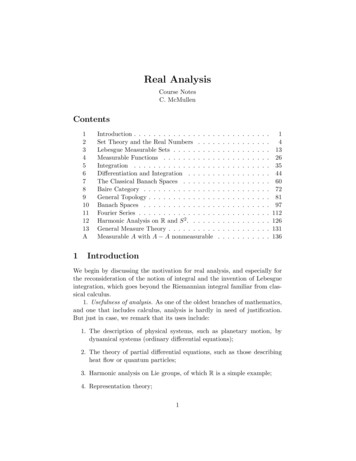
6BORIS BOTVINNIK1. Important examples of topological spaces1.1. Euclidian space, spheres, disks. The notations Rn , Cn have usual meaning throughout the course. The space Cn is identified with R2n by the correspondence(x1 iy1 , . . . , yn ixn ) (x1 , y1, . . . , xn , yn ).The unit sphere in Rn 1 centered in the origin is denoted by S n , the unit disk in Rn by D n ,and the unit cube in Rn by I n . Thus S n 1 is the boundary of the disk D n . Just in case wegive these spaces in coordinates:S n 1 {(x1 , . . . , xn ) Rn x21 · · · x2n 1} ,(1)Dn {(x1 , . . . , xn ) Rn x21 · · · x2n 1} ,In {(x1 , . . . , xn ) Rn 0 xj 1, j 1, . . . , n} .The symbol R is a union (direct limit) of the embeddingsR1 R2 · · · Rn · · · .Thus a point x R is a sequence of points x (x1 , . . . , xn , . . .), where xn R and xj 0for j greater then some k . Topology on R is determined as follows. A set F R isclosed, if each intersection F Rn is closed in Rn . In a similar way we define the spaces C and S .Exercise 1.1. Let x(1) (a1 , 0, . . . , 0, . . .), . . ., x(n) (0, 0, . . . , an , . . .), . . . be a sequence ofelements in R . Prove that the sequence x(n) converges in R if and only if the sequenceof numbers {an } is finite.Probably you already know the another version of infinite-dimensionalPreal space, namely theHilbert space ℓ2 (which is the set of sequences {xn } so that the series n xn converges). Thespace ℓ2 is a metric space, where the distance ρ({xn } , {yn }) is defined aspP2ρ({xn } , {yn }) n (yn xn ) .Clearly there is a natural map R ℓ2 .Remark. The optional exercises are labeled by .Exercise 1.2. Is the above map R ℓ2 homeomorphism or not?Consider the unit cube I in the spaces R , ℓ2 , i.e. I {{xn } 0 xn 1 }.Exercise 1.3. Prove or disprove that the cube I is compact space (in R or ℓ2 ).We are going to play a little bit with the sphere S n .Claim 1.1. A punctured sphere S n \ {x0 } is homeomorphic to Rn .Proof. We construct a map f : S n \ {x0 } Rn which is known as stereographic projection.Let S n be given as above (1). Let the point x0 be the North Pole, so it has the coordinates(0, . . . , 0, 1) Rn 1 . Consider a point x (x1 , . . . , xn 1 ) S n , x 6 x0 , and the line
NOTES ON THE COURSE “ALGEBRAIC TOPOLOGY”7going through the points x and x0 . A directional vector of this line may be given as v ( x1 , . . . , xn , 1 xn 1 ), so any point of this line could be written as(0, . . . , 0, 1) t( x1 , . . . , xn , 1 xn 1 ) ( tx1 , . . . , txn , 1 t(1 xn 1 )).The intersection point of this line and Rn {(x1 , . . . , xn , 0)} Rn 1 is determined byvanishing the last coordinate. Clearly the last coordinate vanishes if t 1 x1n 1 . The mapf : S n \ {pt} Rn is given by xnx1f : (x1 , . . . , xn 1 ) 7 ,.,,0 .1 xn 11 xn 1The rest of the proof is left to you.Figure 1. Stereographic projection We define a hemisphere S n x21 · · · x2n 1 1 & xn 1 0 .Exercise 1.4. Prove the that S n and D n are homeomorphic.1.2. Real projective spaces. A real projective space RPn is a set of all lines in Rn 1 goingthrough 0 Rn 1 . Let ℓ RPn be a line, then we define a basis for topology on RPn asfollows:Uǫ (ℓ) {ℓ′ the angle between ℓ and ℓ′ less then ǫ} .Exercise 1.5. A projective space RP1 is homeomorphic to the circle S 1 .Let (x1 , . . . , xn 1 ) be coordinates of a vector parallel to ℓ, then the vector (λx1 , . . . , λxn 1 )defines the same line ℓ (for λ 6 0). We identify all these coordinates, the equivalence classis called homogeneous coordinates (x1 : . . . : xn 1 ). Note that there is at least one xi whichis not zero. LetUj {ℓ (x1 : . . . : xn 1 ) xj 6 0 } RPnThen we define the map fjR : Uj Rn by the formula xj 1xj 1xn 1x1 x2, ,.,, 1,,.,.(x1 : . . . : xn 1 ) xj xjxjxjxiRemark. The map fjR is a homeomorphism, it determines a local coordinate system in RPngiving this space a structure of smooth manifold of dimension n.There is natural map c : S n RPn which sends each point s (s1 , . . . , sn 1 ) S n to theline going through zero and s. Note that there are exactly two points s and s which mapto the same line ℓ RPn .
8BORIS BOTVINNIKWe have a chain of embeddingswe define RP SRP1 RP2 · · · RPn RPn 1 · · · ,n 1 RPnwith the limit topology (similarly to the above case of R ).1.3. Complex projective spaces. Let CPn be the space of all complex lines in the complexspace Cn 1 . In the same way as above we define homogeneous coordinates (z1 : . . . : zn 1 )for each complex line ℓ CPn , and the “local coordinate system”:Ui {ℓ (z1 : . . . : zn ) zi 6 0 } CPn .Clearly there is a homemorphism fiC : Ui Cn 1 .Exercise 1.6. Prove that the projective space CP1 is homeomorphic to the sphere S 2 .Consider the sphere S 2n 1 Cn 1 . Each pointz (z1 , . . . , zn 1 ) S 2n 1 , z1 2 · · · zn 1 2 1of the sphere S 2n 1 determines a line ℓ (z1 : . . . : zn 1 ) CPn . Observe that the pointeiϕ z (eiϕ z1 , . . . , eiϕ zn 1 ) S 2n 1 determines the same complex line ℓ CPn . We havedefined the map g(n) : S 2n 1 CPn .Exercise 1.7. Prove that the map g(n) : S 2n 1 CPn has a property that g(n) 1 (ℓ) S 1for any ℓ CPn .The case n 1 is very interesting since CP1 S 2 , here we have the map g(1) : S 3 S 2where g(1) 1(x) S 1 for any x S 2 . This map is the Hopf map, it gives very importantexample of nontrivial map S 3 S 2 . Before this map was discovered by Hopf, peoplethought that there are no nontrivial maps S k S n for k n (“trivial map” means a maphomotopic to the constant map).Exercise 1.8. Prove that RPn , CPn are compact and connected spaces.Besides the reals R and complex numbers C there are quaternion numbers H. Recall thatq H may be thought as a sum q a ib jc kd, where a, b, c, d R, and the symbolsi, j, k satisfy the identities:i2 j 2 k 2 1, ij ji k, jk kj i, ki ik j.Then two quaternions q1 a1 ib1 jc1 kd1 and q2 a2 ib2 jc2 kd2 may be multipliedusing these identies. The product here is not commutative, however one can choose left orright multiplication to define a line in Hn 1 . A set of all quaternionic lines in Hn 1 is thequaternion projective space HPn .Exercise 1.9. Give details of the above definition. In particular, check that the space HPnis well-defined. Identify the quaternionic line HP1 with some well-known topological space.
NOTES ON THE COURSE “ALGEBRAIC TOPOLOGY”91.4. Grassmannian manifolds. These spaces generalize the projective spaces. Indeed, thespace G(n, k) is a space of all k -dimensional vector subpaces of Rn with natural topology.Clearly G(n, 1) RP1 . It is not difficult to introduce local coordinates in G(n, k). Letπ G(n, k) be a k -plane. Choose k linearly independent vectors v1 , . . . , vk generating πand write their coordinates in the standard basis e1 , . . . , en of Rn : a11 · · · a1n. .A .ak1 · · · aknSince the vectors v1 , . . . , vk are linearly independent there exist k columns of the matrix Awhich are linearly independent as well. In other words, there are indices i1 , . . . , ik so that aprojection of the plane π on the k -plane hei1 , . . . , eik i generated by the coordinate vectorsei1 , . . . , eik is a linear isomorphism. Now it is easy to introduce local coordinates on theGrassmanian manifold G(n, k). Indeed, choose the indices i1 , . . . , ik , 1 i1 · · · ik n,and consider all k -planes π G(n, k) so that the projection of π on the plane hei1 , . . . , eik iis a linear isomorphism. We denote this set of k -planes by Ui1 ,.,ik .Exercise 1.10. Construct a homeomorphism fi1 ,.,ik : Ui1 ,.,ik Rk(n k) .The result of this exercise shows that the Grassmannian manifold G(n, k) is a smooth manifoldof dimension k(n k). The projective spaces and Grassmannian manifolds are very importantexamples of spaces which we will see many times in our course.Exercise 1.11. Define a complex Grassmannian manifold CG(n, k) and construct a localcoordinate system for CG(n, k). In particular, find its dimension.We have a chain of spaces:G(k, k) G(k 1, k) · · · G(n, k) G(n 1, k) · · · .Let G( , k) be the union (inductive limit) of these spaces. The topology of G( , k) isgiven in the same way as to R : a set F G( , k) is closed if and only if the intersectionF G(n, k) is closed for each n. This topology is known as a topology of an inductive limit.Exercise 1.12. Prove that the Grassmannian manifolds G(n, k) and CG(n, k) are compactand connected.1.5. Flag manifolds. Here we just mention these examples without further considerations(we are not ready for this yet). Let 1 k1 · · · ks n 1. A flag of the type (k1 , . . . , ks )is a chain of vector subspaces V1 · · · Vs of Rn such that dim Vi ki . A set of flags ofthe given type is the flag manifold F (n; k1 , . . . , ks ). Hopefully we shall return to these spaces:they are very interesting and popular creatures.1.6. Classic Lie groups. The first example here is the group GL(Rn ) of nondegeneratedlinear transformations of Rn . Once we choose a basis e1 , . . . , en of Rn , each element A GL(Rn ) may be identified with an n n matrix A with det A 6 0. Clearly we may identify2the space of all n n matrices with the space Rn . The determinant gives a continuous22function det : Rn R, and the space GL(Rn ) is an open subset of Rn :2GL(Rn ) Rn \ det 1 (0).
10BORIS BOTVINNIKIn particular, this identification defines a topology on GL(Rk ). In the same way one may2construct an embedding GL(Cn ) Cn . The orthogonal and special orthogonal groups O(k),SO(k) are subgroups of GL(Rk ), and the groups U(k), SU(k) are subgroups of GL(Ck ).(Recall that O(n) (or U(n)) is a group of those linear transformations of Rn (or Cn ) whichpreserve a Euclidian (or Hermitian) metric on Rn (or Cn ), and the groups SO(k) and SU(k)are subgroups of O(k) and U(k) of matrices with the determinant 1.)Exercise 1.13. Prove that SO(2) and U(1) are homeomorphic to S 1 , and that SO(3) ishomeomorphic to RP3 .Hint: To prove that SO(3) is homeomorphic to RP3 you have to analyze SO(3): the keyfact is the geometric description of an orthogonal transformation α SO(3), it is given byrotating a plane (by an angle ϕ) about a line ℓ perpendicular to that plane. You should use theline ℓ and the angle ϕ as major parameters to construct a homeomorphism SO(3) RP3 ,where it is important to use a particular model of RP3 , namely a disk D 3 where one identifiesthe opposite points on S 2 D 3 D 3 .Exercise 1.14. Prove that the spaces O(n), SO(n), U(n), SU(n) are compact.Exercise 1.15. Prove that the space O(n) has two path-connected components, and that thespaces SO(n), U(n), SU(n) are path-connected.Exercise 1.16. Prove that each matrix A SU(2) may be presented as: α βA , where α, β C, α 2 β 2 1 β̄ ᾱUse this presentation to prove that SU(2) is homeomorphic to S 3 .It is important to emphasize that the classic groups O(n), SO(n), U(n), SU(n) are allmanifolds, i.e. for each point α there there exists an open neighborhood homeomorphic to aEuclidian space.Exercise 1.17. Prove that the space for any point α SO(n) there exists an open neighborhood homeomorphic to the Euclidian space of the dimension n(n 1).2Exercise 1.18. Prove that the spaces U(n), SU(n) are manifolds and find their dimension.The next set of examples is also very important.1.7. Stiefel manifolds. Again, we consider the vector space Rn . We call vectors v1 , . . . , vka k -frame if they are linearly independent. A k -frame v1 , . . . , vk is called an orthonormalk -frame if the vectors v1 , . . . , vk are of unit length and orthogonal to each other. The spaceof all orthonormal k -frames in Rn is denoted by V (n, k). There are analogous complex andquaternionic versions of these spaces, they are denoted as CV (n, k) and HV (n, k) respectively. Here is an exercise where your knowledge of basic linear algebra may be crucial:Exercise 1.19. Prove the following homeomorphisms: V (n, n) O(n), V (n, n 1) SO(n), CV (n, n) U(n), CV (n, n 1) SU(n), V (n, 1) S n 1 , CV (n, 1) S 2n 1 ,HV (n, 1) S 4n 1 .
NOTES ON THE COURSE “ALGEBRAIC TOPOLOGY”11We note that the group O(n) acts on the spaces V (n, k) and G(n, k): indeed, if α O(n)and v1 , . . . , vk is an orthonormal k -frame, then α(v1 ), . . . , α(vk ) is also an orthonormal k frame. As for the Grassmannian manifold, one can easily see that α(Π) is a k -dimensionalsubspace in Rn if Π is.The group O(n) contains a subgroup O(j) which acts on Rj Rn , where Rj he1 , . . . , ej iis generated by the first j vectors e1 , . . . , ej of the standard basis e1 , . . . , en of Rn . SimilarlyU(n) acts on the spaces CG(n, k) and CV (n, k), and U(j) is a subgroup of U(n).Exercise 1.20. Prove the following homeomorphisms:(a) S n 1 SO(n)/SO(n 1), O(n)/O(n 1) (b) S 2n 1 U(n)/U(n 1) SU(n)/SU(n 1),(c) G(n, k) O(n)/O(k) O(n k),(c) CG(n, k) U(n)/U(k) U(n k).We note here that O(k) O(n k) is a subgroup of O(n) of orthogonal matrices with twodiagonal blocks of the sizes k k and (n k) (n k) and zeros otherwise.There is also the following natural action of the orthogonal group O(k) on the Stieffelmanifold V (n, k). Let v1 , . . . , vk be an orthonormal k -frame then O(k) acts on the spaceV hv1 , . . . , vk i, in particular, if α O(k), then α(v1 ), . . . , α(vk ) is also an orthonormalk -frame. Similarly there is a natural action of U(k) on CV (n, k).Exercise 1.21. Prove that the above actions of O(k) on V (n, k) and of U(k) on CV (n, k)are free.Exercise 1.22. Prove the following homeomorphisms:(a) V (n, k)/O(k) G(n, k),(b) CV (n, k)/U(k) CG(n, k).ppThere are obvious maps V (n, k) G(n, k), CV (n, k) CG(n, k) (where each orthonormal k -frame v1 , . . . , vk maps to the k -plane π hv1 , . . . , vk i generated by this frame). It iseasy to see that the inverse image p 1 (π) may be identified with O(k) (in the real case) andU(k) (in the complex case). We shall return to these spaces later on. In particular, we shalldescribe a cell-structure of these spaces and compute their homology and cohomology groups.1.8. Surfaces. Here I refer to Chapter 1 of Massey, Algebraic topology, for details. I wouldlike for you to read this Chapter carefully even though most of you have seen this materialbefore. Here I briefly remind some constructions and give exercises. The section 4 of thereffered Massey book gives the examples of surfaces. In particular, the torus T 2 is describedin three different ways:(a) A product S 1 S 1 .
12BORIS BOTVINNIK(b) A subspace of R3 given by:nop(x, y, z) R3 ( x2 y 2 2)2 z 2 1 .(c) A unit square I 2 {(x, y) R2 0 x 1, 0 y 1 } with the identification:(x, 0) (x, 1) (0, y) (1, y) for all 0 x 1,0 y 1.Exercise 1.23. Prove that the spaces described in (a), (b), (c) are indeed homeomorphic.bbaaaba bT2Figure 2. Torus and projective planeRP2The next surface we want to become our best friend is the projective space RP2 . Earlier wedefined RP2 as a space of lines in R3 going through the origin.Exercise 1.24. Prove that the projective plane RP2 is homeomorphic to the following spaces:(a) The unit disk D 2 {(x, y) R2 x2 y 2 1} with the opposite points (x, y) ( x, y) of the circle S 1 {(x, y) R2 x2 y 2 1} D 2 have been identified.(b) The unit square, see Fig. 3, with the arrows a and b identified as it is shown.(c) The Mëbius band which boundary (the circle) is identified with the boundary of thedisk D 2 , see Fig. 3.baaaabMëD2Figure 3The Klein bottleHere the Mëbius band is constructed from a square by identifying the arrows a. The Kleinbottle Kl2 may be described as a square with arrows identified as it is shown in Fig. 3.Exercise 1.25. Prove that the Klein bottle Kl2 is homeomorphic to the union of two Mëbiusbands along the circle.Massey carefully defines connected sum S1 #S2 of two surfaces S1 and S2 .Exercise 1.26. Prove that Kl2 #RP2 is homeomorphic to RP2#T 2 .Exercise 1.27. Prove that Kl2 #Kl2 is homeomorphic to Kl2 .Exercise 1.28. Prove that RP2 #RP2 is homeomorphic to Kl2 .
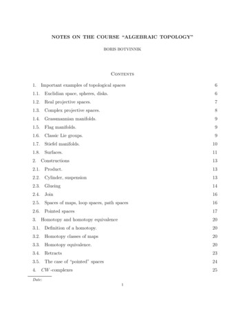
NOTES ON THE COURSE “ALGEBRAIC TOPOLOGY”132. Constructions2.1. Product. Recall that a product X Y of X , Y is a set of pairs (x, y), x X, y Y .If X , Y are topological spaces then a basis for product topology on X Y is given by theproducts U V , where U X , V Y are open. Here are the first examples:Example. The torus T n S 1 · · · S 1 . Note that the torus T n may be identified withU(1) · · · U(1) U(n) (diagonal orthogonal complex matrices).Exercise 2.1. Consider the surface X in S 5 , given by the equationx1 x6 x2 x5 x3 x4 0(where S 5 R6 is given by x21 · · · x26 1). Prove that X S2 S2 .Exercise 2.2. Prove that the space SO(4) is homeomorphic to S 3 RP3 .Hint: Consider carefully the map SO(4) S 3 SO(4)/SO(3) and use the fact that S 3has a natural group structure: it is a group of unit quaternions. It should be emphasized thatit is not true that SO(n) S n 1 SO(n 1) if n 4.prXprYWe note also that there are standard projections X Y X and X Y Y , and togive a map f : Z X Y is the same as to give two maps fX : Z X and fY : Z Y .2.2. Cylinder, suspension. Let I [0, 1] R. The space X I is called a cylinder overX , and the subspaces X {0}, X {1} are the bottom and top “bases”. Now we willconstruct new spaces out of the cylinder X I .Remark: quotient topology. Let “ ” be an equivalence relation on the topological spaceX . We denote by X/ the set of equivalence classes. There is a natural map (not continuosso far) p : X X/ . We define the following topology on X/ : the set U X/ isopen if and only if p 1 (U) is open. This topology is called a quotient topology.The first example: let A X be a closed set. Then we define the relation “ ” on X asfollows ([ ] denote an equivalence class): {x} if x / A,[x] A if x A.The space X/ is denoted by X/A.The space C(X) X I/X {1} is a cone over X . A suspention ΣX over X is the spaceC(X)/X {0}.Exercise 2.3. Prove that the spaces C(S n ) and ΣS n are homeomorphic to D n 1 and S n 1respectively.Here is a picture of these spaces:
14BORIS BOTVINNIKX IC(X)ΣXFigure 42.3. Glueing. Let X and Y be topological spaces, A Y and ϕ : A X be a map. Weconsider a disjoint union X Y , and then we identify a point a A with the point ϕ(a) X .The quotient space X Y / under this identification will be denoted as X ϕ Y , and thisprocedure will be called glueing X and Y by means of ϕ. There are two special cases of thisconstruction.Let f : X Y be a map. We identify X with the bottom base X {0} of the cylinderX I . The space X I f Y Cyl(f ) is called a cylinder of the map f . The spaceC(X) f Y is called a cone of the map f . Note that the space Cyl(f ) contains X and Y assubspaces, and the space C(f ) contains X 1111100000000000000000001111111111111111111YCyl(f )C(f )Figure 5Let f : S n RPn be the (we have studied before) map which takes a vector v S n to theline ℓ h v i spanned by v .D n 1C(S n )fRPnFigure 6Claim 2.1. The cone C(f ) is homeomorphic to the projective space RPn 1 .Proof (outline). Consider the cone over S n , clearly C(S n ) D n 1 (Exercise 2.3). Nown 1nthe cone C(f ) is a disk Dwith the opposite points of S identified, see Fig. 6.
NOTES ON THE COURSE “ALGEBRAIC TOPOLOGY”15In particular, a cone of the map f : S 1 S 1 RP1 (given by the formula eiϕ 7 e2iϕ )coincides with the projective plane RP2 .Exercise 2.4. Prove that a cone C(h) of the Hopf map h : S 2n 1 CPn is homeomorphicto the projective space CPn 1 .Here is the construction which should help you with Exercise 2.4. Let us take one morelook at the Hopf map h : S 2k 1 CPk : we take a point (z1 , · · · , zk 1) S 2k 1 , (where z1 2 · · · zk 1 2 1), then h takes it to the line (z1 : · · · : zk 1 ) CPk . Moreover′h(z1 , · · · , zk 1 ) (z1′ , · · · , zk 1) if and only if zj′ eiϕ zj . Thus we can identify CPk withthe following quotient space:(2)CPk S 2k 1 / ,where (z1 , · · · , zk 1) (eiϕ z1 , · · · , eiϕ zk 1 ).Now consider a subset of lines in CPk where the last homogeneous coordinate is nonzero:Uk 1 {(z1 : · · · : zk 1 ) zk 1 6 0} .We already know that Uk 1 is homeomorphic to Ck by means of the map zkz1(z1 : · · · : zk 1 ) 7 zk 1, . . . , zk 1Now we use (2) to identify Uk 1 with an open disk D 2k Ck as follows. Let us think aboutUk 1 S 2k 1 / as above. Let ℓ Uk 1 . Choose a point (z1 , · · · , zk 1 ) S 2k 1 representingℓ. Then we have that z1 2 · · · zk 1 2 1, and zk 1 6 0.A complex number zk 1 has a unique representation zk 1 reiα , where r zk 1 . Noticethat 0 r 1. Then the point(e iα z1 , e iα zk · · · , e iα zk 1 ) (e iα z1 , e iα zk · · · , r) S 2k 1represents the same line ℓ Uk 1 . Moreover, this representation is unique. We have: z1 2 · · · zk 2 1 r 2 2k 12k 1 Ck of radius 1 r 2 . The union of the spheres S which describes the sphere S 1 r 21 r 2over 0 r 1 is nothing but an open unit disk in Ck . Then we notice that we can let zk 1to be equal to zero: zk 1 0 corresponds to the points(z1 , · · · , zk , 0) S 2k 1 with z1 2 · · · zk 2 1,i.e.the sphere S 2k 1 Ck modulo the equivalence relation (z1 , · · · , zk , 0) (eiϕ z1 , · · · , eiϕ zk , 0). This is nothing but the projective space CPk 1 . We summarize ourconstruction:Lemma 2.1. There is a homeomorphismCPk D 2k / ,where (z1 , · · · , zk ) (z1′ , · · · , zk′ ) if and only if z1 2 · · · zk 2 1, z1′ 2 · · · zk′ 2 1, andzj′ eiϕ zjfor all j 1, . . . , k.
16BORIS BOTVINNIK2.4. Join. A join X Y of spaces X Y is a union of all linear paths Ix,y starting at x Xand ending at y Y ; the union is taken over all points x X and y Y . For example,a joint of two intervals I1 and I2 lying on two non-parallel and non-intersecting lines isa tetrahedron: A formal definition of X Y is the following. We start with the productI2I1Figure 7X Y I : here there is a linear path (x, y, t), t I for given points x X , y Y . Thenwe identify the following points:(x, y ′ , 1) (x, y ′′, 1) for any x X, y ′, y ′′ Y ,(x′ , y, 0) (x′′ , y, 0) for any x′ , x′′ X, y Y .Exercise 2.5. Prove the homeomorphisms(a) X {one point} C(X);(b) X {two points} Σ(X);n k 1(c) S n S k S. Hint: prove first that S 1 S 1 S3 .2.5. Spaces of maps, loop spaces, path spaces. Let X , Y are topological spaces. Weconsider the space C(X, Y ) of all continuous maps from X to Y . To define a topology ofthe functional space C(X, Y ) it is enough to describe a basis. The basis of the compact-opentopology is given as follows. Let K X be a compact set, and O Y be an open set. Wedenote by U(K, O) the set of all continuous maps f : X Y such that f (K) Y , this is(by definition) a basis for the compact-open topology on C(X, Y ).Examples. Let X be a point. Then the space C(X, Y ) is homeomorphic to Y . If X be aspace consisting of n points, then C(X, Y ) Y · · · Y (n times).Let X , Y , and Z be Hausdorff and locally compact1 topological spaces. There is a naturalmapT : C(X, C(Y, Z)) C(X Y, Z),given by the formula: {f : X C(Y, Z)} {(x, y) (f (x))(y)} .Exercise 2.6. Prove that the map T : C(X,
NOTES ON THE COURSE “ALGEBRAIC TOPOLOGY” 3 8.3. Relative homotopy groups 61 9. Fiber bundles 65 9.1. First steps toward fiber bundles 65 9.2. Constructions of new fiber bundles 67 9.3. Serre fiber bundles 70 9.4. Homotopy exact sequence of a fiber bundle 73 9.5. More on the group