WIXLIB

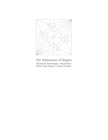
The Mathematics of Origamiand CP x–ABx 12x 1 x– .333Thus, 4 CBT 4P SC andand y we gety x 1 y2x 13x 13 BTCP ,CTCS2x 1,x 12x2 x–1. Combining this and the equation for y found earlier,3x2x2 x–1x2 2x .2x 23xAfter cross multiplying, the solution simplifies to x3 2. Therefore, x [2] 32.Origami is shown to be far more powerful than compass and straightedgeas a method of construction, as these problems previously proven unsolvablethrough the use of compass and straightedge were proved solvable throughthe use of origami. However, squaring the circle, or constructing a squarewhose area is the same as a given circle, is impossible to construct throughorigami because π would need to be constructed. Pi is a transcendentalnumber, and thus not the root of a polynomial with integer coefficients(only polynomial equations with rational coefficients can be solved withorigami—π is irrational). However, curved (non-flat) creases can allow forthe construction of non-algebraic numbers. An approximation for π can beconstructed by valley-folding a semicircle (centered at a given point A) alongthe long side of a strip of paper, then making an angle of 45 or less by valleycreasing from one end of the semicircle (labeled B). An example of a valleyfold can be seen in fig. 2.1. Once the crease is folded flat and the semicircleis folded, part of a cone should be formed. Then, the raw edge of the paperpositioned by the 45 (or less) crease should slide into the semicircle. If thepoint where the raw edge touches the other end of the semicircle is creasedand labeled C, the length of BC is the perimeter of the semicircle. Thus, ifthe semicircle’s radius AB 1, BC/AB π, implying BC π (to abouttwo decimal places). [12]The methods used in this construction could be formalized as follows:“Given a line L and a curve C, we can align L onto C or vice-versa.” This issimilar to the third Huzita axiom—“Given two lines l1 and l2 , we can foldline l1 onto l2 ,” though nothing is mentioned about creasing to place L ontoC, only that they can be aligned onto each other. [12]7

The Mathematics of OrigamiWhen discussing origami constructible numbers, a few concepts mustfirst be defined. We will begin with two points, p0 and p1 , and define thedistance between them, p0 p1 , to be 1.Definition 1.1. A line l is constructible if a fold can be formed along linel.Definition 1.2. A point p is constructible if two lines can be constructedthat cross at point p.Definition 1.3. A number α is constructible if two points can be constructeda distance α apart. [7]In order to establish the Cartesian plane, we must first create a vectorfrom p0 to p1 as the initial basis vector e1 . Then, to find the second basisvector e2 , we construct a line segment with a magnitude equal to that of e1extending at a right angle from point p0 to e1 . The endpoint of this linesegment will be denoted p01 , reaffirming the line segment’s unit length 1.Thus, e2 , the second basis vector, will extend from p0 to p01 . [7]Function 1. Given two points p0 and p1 , construct a third point p01 adistance p0 p1 from point p0 such that p0 p01 p0 p1 . [7]The construction of these functions involves the use of the original sevenHuzita-Justin Axioms.Using Axiom 1, construct the line l1 passing through p0 and p1 .Using Axiom 4, construct the line l2 l1 passing through p1 .Using Axiom 4, construct the line l3 l1 passing through p0 .Using Axiom 3, construct the line l4 placing l1 onto l2 .The point constructed upon the crossing of l3 and l4 is the point p01 . [7]Proof. Since p01 lies on l3 which, by definition, is perpendicular to l1 andconstructible by Axiom 4, p0 p1 is perpendicular to p0 p01 . The acute angleformed by l1 and l4 must be equal to that which is created by l2 and l4 , sincel1 was placed onto l2 when forming l4 . The angle created by l1 and l2 isbisected by l4 . Lines l2 and l3 are parallel, and thus both are perpendicularto l1 . By alternate interior angles, the acute angle made by l2 and l4 is equalto the angle formed by l3 and l4 . Finally, since p0 p1 p01 p0 p01 p1 , 4p1 p0 p010is an isosceles triangle, such that p0 p1 p0 p1 . [7]Function 2. Given two points p0 and p1 , a third point p2 can beconstructed such that p2 is collinear with p0 and p1 , and thus p0 p1 p1 p2 .[7]8

The Mathematics of OrigamiUse Function 1 to create p01 from p0 and p1 such that p1 p0 p01 is aright angle. From Function 1, l1 (through p0 and p1 ), l2 (through p1 andperpendicular to l1 ), and l3 (through p0 and perpendicular to l1 ) have beenformed.Use Axiom 4 to create the line l5 l3 through p01 .Use Axiom 3 to create the line l6 placing l5 onto l2 .The point constructed upon the crossing of l1 and l6 is p2 . [7]Proof. The points p0 , p1 , and p2 are collinear, since they all lie on l1 . Bycongruent triangles 4p1 p0 p01 4p2 p1 p3 having three equivalent angles andone equivalent side, where the intersection of l2 and l5 is p3 , p0 p1 p1 p2 .[7]All positive and negative integers have been shown to be constructiblealong the axes e1 and e2 (whose constructions are described earlier). Thus,any point in ZxZ is constructible by finding the intersection of a perpendicular extended from integers constructed on each axis. We will now movefrom ZxZ to QxQ. [7]Function 3. Given two constructible numbers α and β, we can constructαβ , their ratio. [7]Extending from p0 , construct a point pa a distance α along the e1 axisand a point pb a distance β along the e2 axis.Use Axiom 4 to construct the line l1 p0 pa through pa .Use Axiom 5 to create the line l2 passing through p0 and placing pb ontol1 .Use Axiom 4 to create the line l3 l2 passing through pb . Denote theintersection of l1 and l3 point p2 . Now p0 p2 β.Use Axiom 1 to form the line l4 passing through p0 and p2 .Use Function 1 to form p01 one unit along the e2 axis.Use Axiom 5 to construct the line l5 passing through p0 and placing p01onto l4 .Use Axiom 4 to create the line l6 l5 passing through p01 . Denote theintersection of l4 and l6 point p3 . Thus, p0 p3 1.Use Axiom 1 to form the line l0 through p0 and p1 .Use Axiom 4 to construct the line l7 l0 passing through p3 . Denotethe intersection of l0 and l7 point pr .Thus, p0 pr αβ . [7]Proof. Denote the intersection of l2 and l3 as px . The lengths of pb px andpx p2 must be equivalent, as they are able to be superimposed upon each9

The Mathematics of Origami 1βαββ1ααFigure 1.5: Ratio Construction and Creases Involvedother. Next, 4p0 px pb and 4p0 px p2 both share the side p0 px , thus by sideangle-side, the two triangles are congruent. Similarly, it can be proven that p0 p3 1. In addition, 4p0 pr p3 4p0 pa p2 . These two triangles are righttriangles, and both share an angle—thus, all three angles corresponding withone another are equal, and the triangles are similar. Therefore, the ratio p0 pa p0 pr of corresponding sides is also equal, and . Since p0 pa α, p0 p2 p0 p3 p0 pr α p0 pr . [7] p0 p2 β, and p0 p3 1, by substitution, β1Thus, by extending a perpendicular from the intersection of a ratio ofintegers constructed on each axis, any point in Q2 can be constructed [7].It has been proven that the division of any two constructible numbers ispossible. Since it is apparent we are able to construct the rational numbers, we will continue to prove that origami constructible numbers form afield. The rationals form a field, and thus all we know how to constructforms a field. To ensure the structure of the field is maintained even if constructible non-rational numbers are discovered, we must determine if theorigami constructible numbers are closed under addition, subtraction, andmultiplication, along with the previously proven division. [7]Function 4. Given two constructible numbers α and β, we can constructtheir sum α β or their difference α–β. [7]Create the point pa extending from p0 a distance α along the e1 axis.Create the point pb extending from pa a distance β along the e1 axisin the same direction as e1 for addition and in the opposite direction forsubtraction.Ultimately, p0 pb α β (or α–β). [7]Proof. The appropriate sum or difference has obviously been constructed ifany previously constructible points based from pa can indeed be constructed.10

The Mathematics of OrigamiTo construct the necessary unit length based from point pa , begin by constructing the axes using Axiom 1 to form the line l1 p0 pa and the linel2 p0 p01 . Therefore, l1 is perpendicular to l2 .Use Axiom 4 to construct the line l3 perpendicular to l2 through pointp01 , and again to form the line l4 perpendicular to l1 through pa . Denote theintersection of l3 and l4 point p0a .Use Axiom 3 to construct the line l5 placing l3 onto l4 . Denote theintersection of l1 and l5 point p2 .The lines l1 and l3 are one unit apart and the triangle created is isosceles(by the proof of Function 2)—thus, p2 is one unit away from pa . The numberβ previously constructible from p0 using p1 is now constructible using pa andp2 . [7]Function 5. Given two constructible numbers α and β, we can constructαβ, their product. [7]Because of the repetitive nature of these constructions, these steps willnot be listed here. All that must be done to construct the multiplication ofα and β is divide α by the reciprocal of β—the construction of such division1has already been proven. Using Function 3, we divide one by β to get ,β1then divide α by . After simplification, the result is equal to αβ. [7]βIt has been proven that the set of constructible numbers is closed under addition, subtraction, multiplication, and division—thus, it can be concluded that the set of constructible numbers forms a field. Ultimately, thefield of origami constructible numbers is closed under taking both squareroots and cube roots. The construction of the square root of any constructible number implies the field of origami constructible numbers contains the field of compass and straightedge constructible numbers. For convenience, the steps and proofs of these constructions will not be included,but referring to Shepherd Engle’s paper entitled “Origami, Algebra, andthe Cubic” will give a thorough understanding of the constructions andtheir corresponding proofs. The originally unsolvable (through compass andstraightedge) problems of trisecting an angle and doubling the cube, as described earlier, were discovered to be easily solvable through origami. Thisis due in part to trisecting an angle reducing to solving a cubic equation,and doubling the cube reducing to constructing the cube root of two [7].A good route to pursue in the future would look at the efficiency oforigami constructions versus other construction tools. Problems relating tothis topic include the study of the existence of constructions being alge-11

The Mathematics of Origamibraically and geometrically optimal. Determining the uniqueness and optimality of a given construction remains an open problem. In addition, onemay consider forming relations satisfied by the degrees, levels, and orders ofconstructions [21].1.2Lill’s methodIn 1868, Eduard Lill published a geometric method for finding real roots ofpolynomials. Margherita Beloch realized, in 1936, that this method couldbe adapted to paper folding, allowing one to find roots of polynomials withrational coefficients by making a series of folds [13]. With single-fold axioms,polynomials of degree 3 or less can be solved. In general, if we allow nsimultaneous folds, we can solve polynomials of degree up to n 2 [13]. See[22] for more information on Lill’s Method adapted for origami.Before looking at Lill’s method, we must learn about Horner’s form ofa polynomial. For a polynomial written in standard form asp(x) an xn an 1 xn 1 · · · a1 x a0 ,Horner’s form isp(x) (((an x an 1 )x an 2 )x · · · )x a0 .Horner’s form leads to an efficient algorithm for computing values of a polynomial. For finding the value p(x0 ), compute a series of values:bn : anbn 1 : bn x0 an 1.b0 : b1 x0 a0 .Then b0 p(x0 ).This algorithm provides the basis for Lill’s method. We’ll start with anexample of a cubic equation; considerf (x) a3 x3 a2 x2 a1 x a0 .We will represent this graphically with a right-angled path, shown in figure1.6(a). To construct the path, start at the origin and walk a distance a3vertically. Then turn clockwise 90 and walk a distance a2 . (Note that if a2is negative, you will walk backwards.) For each new coefficient, repeat thisprocess of turning 90 and walking for a distance given by the coefficient.12

The Mathematics of OrigamiFigure 1.6: The outer right-angled path has lengths determined by the coefficients. In (a),the endpoints of the inner and outer paths coincide. In (b), they do not.Now, create a second right-angled path, represented in 1.6(a) as a dottedline starting at the origin O. Launch the line at an angle θ and any timeyou intersect the original right-angled path, reflect at an angle of 90 . Now,vary the angle θ until the endpoints of both paths coincide at s. When theendpoints coincide, tan θ is a root of f ; so f ( tan θ) 0.Why does this occur? Let’s consider the length l between points s and tin fig. 1.6(b). In order to find this length, first note that the triangles Op1 p2 ,p2 p3 p4 , and p4 p5 t are all similar. Now we’ll find the length of segment p1 p2 .Simple trigonometry tells us that it is a3 tan θ. Next, the length of p2 p3 isa2 a3 tan θ.Now, let’s find the length of p4 p5 . In a similar manner to above, we learnthat it isa1 (a2 a3 tan θ) tan θ.And similarly, the length of l isa0 (a1 (a2 a3 tan θ) tan θ) tan θ.Note that when this length is 0, we have0 a0 (a1 (a2 a3 tan θ) tan θ) tan θand we have constructed Horner’s form of the polynomial f , and so when sand t coincide, tan θ is a root of f !How can we adapt this method to folding? It is fairly simple. We definea unit length on the paper to be the length between some points p1 and p2 .13

The Mathematics of OrigamiAs long as the coefficients are rational (or in general algebraic if we allowsimultaneous folds), we can construct segments with the lengths determinedby the coefficients. Thus we can construct the outer right-angled path.Note that for a polynomialp(x) an xn an 1 xn 1 · · · a1 x a0 ,we can divide it by an without changing the roots, giving us the monicpolynomialan 1 n 1a1a0p(x) xn x ··· x .anananUsing a monic polynomial with origami has the advantage that the firstsegment in the outer right-angled path has unit length. This means, inparticular, that the length p1 p2 will (up to sign) be a root of the polynomial,sincep1 p2 an tan θ tan θ.So solving a polynomial with origami means constructing segments withlength equal to the (real) roots of the polynomial. Constructing the outerright-angled path is simple using Axiom 4, which allows us to construct linesperpendicular to lines we have already. Creating the inner path is moreinvolved. In the case of a cubic equation, using Axiom 6 will be necesaryto find the proper lines to create the path. Once we have created the innerright-angled path, we have a length equal to a root of the polynomial.2General FoldabilityThe above constructions, for the most part, rely on making a single creaseand then unfolding it, to use the mark it left on the paper. However, mostorigami does not work this way - after making a fold, it stays, and then wefold over it. Here we discuss the mathematical formalism for this kind offolding.One of the best ways to study origami is through studying crease patterns. Intuitively, a crease pattern is obtained by folding an origami model,and then unfolding the paper. The lines left on the paper by the folds formthe crease pattern. We will only consider crease patterns that use straightline creases. While it is possible to fold origami using curved creases, thesetypes of models are much less common and are more difficult to study mathematically and curved creases will not appear in any of the topics we consider.14

The Mathematics of OrigamiDefinition 2.1 (Crease Pattern). A crease pattern is a pair (C, R) whereC is a set of line segments that intersect only at their endpoints and R,representing the piece of paper, is a closed connected subset of R2 , s.t. C R C. An intersection of creases is called a vertex. Note that intersectionsoccurring on the boundary of R will not be considered vertices.This definition of a crease pattern is inspired by [23]. For an example ofa crease pattern, see fig. 2.2(a), which is the crease pattern for the commonbird base form.Generally, we will consider origami using a square piece of paper paper.Note that a crease pattern alone does not capture all of the relevantinformation about an origami model. Every crease can fold upwards ordownwards. These are called valley folds and a mountain folds. We depictvalley folds with dashed lines and mountain folds with dash-dotted lines, asshown in fig. 2.1.Figure 2.1: A mountain fold with a dash-dotted line, and a valley fold with a dashed line.Definition 2.2. A mountain-valley assignment of a crease pattern C {V, E} is a many-to-one mapping E {M, V }.Fig. 2.2(a) is the crease pattern for the bird base, and (b) is the birdbase with a mountain valley assignment.Applying a different mountain-valley assignment to the same crease pattern leads to a different folded form. Note that for a given crease pattern,some assignments may by (flat) foldable while others may not be.When we fold an origami model, we don’t rip the paper or stretch it. Inorder to capture this notion, we define a folding.Definition 2.3 (Folding). A folding of a crease pattern (C, R) is an assignment of angles to each crease, such that the paper, when folded with the15

The Mathematics of OrigamiFigure 2.2: A bird base crease pattern, both assigned and unassigned.angles at the creases, does not rip or stretch, and the faces of the final formare flat.In general, we consider folding to take place in an arbitrary number ofdimensions in order to avoid the paper self-intersecting. Sometimes, as infig 2.3, we can have a folding in three dimensions where the paper selfintersects. This does not correspond to how paper behaves in real life. Toavoid avoid this problem we define a valid folding.Figure 2.3: A valid folding on the left, and invalid on the right, for the same crease pattern.Definition 2.4 (Valid Folding). A valid folding is a folding that does notcause the paper to self-intersect, when projected into R3 by ignoring all higherdimensions.See fig. 3.5 for an example of a crease pattern that has no valid folding,but that can be folded flat if the paper is allowed to self-intersect.Note that the definitions of folding and valid folding do not apply to flatfoldings, but only to foldings in Rn .16

The Mathematics of Origami2.1Foldings and Knot TheoryThe following theorem was inspired by a comment made by Jason Ku (MIT)in his presentation of an origami hole-filling algorithm at JMM 2016. Askedif his algorithm dealt with self-intersection, he said it did not, but that thereare a couple easy initial checks one can perform. “For instance,” he pointedout, “the border of the paper must map to the unknot.”This theorem ties together knot theory and origami, and will hopefullyallow us to gain further insight into ways in which foldings of crease patternsmay or may not self-intersect. An introduction to knot theory sufficient forour purposes can be found in [18].Theorem 2.5. A crease pattern with a given folding is valid if and only ifevery Jordan curve drawn on the unfolded paper gets mapped to the unknotin the final folded form.Proof. First we need to sh

problems are able to be solved using origami. In order to compare these con-struction techniques, we must rst provide geometric axioms, or operations, for creating folds in the plane. 1.1 Axioms of Origami To begin, just as Euclid based his studies on a set of fundamental axioms, or postulates, the mathematics of origami is based on a set of .