Transcription
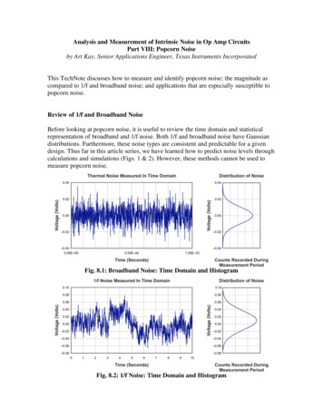
Analysis and Measurement of Intrinsic Noise in Op Amp CircuitsPart VIII: Popcorn Noiseby Art Kay, Senior Applications Engineer, Texas Instruments IncorporatedThis TechNote discusses how to measure and identify popcorn noise; the magnitude ascompared to 1/f and broadband noise; and applications that are especially susceptible topopcorn noise.Review of 1/f and Broadband NoiseBefore looking at popcorn noise, it is useful to review the time domain and statisticalrepresentation of broadband and 1/f noise. Both 1/f and broadband noise have Gaussiandistributions. Furthermore, these noise types are consistent and predictable for a givendesign. Thus far in this article series, we have learned how to predict noise levels throughcalculations and simulations (Figs. 1 & 2). However, these methods cannot be used tomeasure popcorn noise.Fig. 8.1: Broadband Noise: Time Domain and HistogramFig. 8.2: 1/f Noise: Time Domain and Histogram
What is Popcorn Noise?Popcorn noise is a sudden step, or jump, in base current on bipolar transistors, or a step inthreshold voltage on an FET. It got this name because the sound it makes when playedover a speaker resembles the sound of popcorn popping. This noise is also called burstnoise and random telegraph signals (RTS). Popcorn noise occurs at low frequency(typically f 1 kHz). Bursts can happen several times a second or, in some rare cases,may take minutes to occur.Fig. 8.3 shows popcorn noise in the time domain and its associated statistical distribution.Note the distinctive jumps in noise level correspond to peaks in the distribution. Clearly,the distribution associated with popcorn noise in not Gaussian. In fact, the distributionshown in this example is three Gaussian curves placed on top of each other (tri-modeldistribution). This happens because the popcorn noise in this example has three discretelevels. The noise in between bursts is a combination of broadband and 1/f noise. Thus,the noise consists of three different Gaussian distributions from 1/f and broadband noisethat are shifted to different levels by popcorn noise.Fig. 8.3: Popcorn Noise: Time Domain and HistogramWhat Causes Popcorn Noise?Popcorn noise is believed to be caused by charge traps or microscopic defects in thesemiconductor material. Heavy metal atom contaminates are known to cause popcornnoise. Devices with excessive popcorn noise are often closely examined by experts in thefield of failure analysis. Failure analysis searches for microscopic faults that could causepopcorn noise.
Fig. 8.4 shows how a normal transistor compares to one with a crystalline defect.Fig. 8.4: Normal Transistor vs. Transistor with Crystalline DefectHow Common is the Problem?Popcorn noise is related to problems that occur during semiconductor fabrication. Formany modern processes the occurrence of popcorn noise can be relatively small.Generally, there is a lot-to-lot dependency; ie, some lots will have no popcorn noise whileother lots may have a small percentage of contamination. A particularly badsemiconductor lot could have 5% of the devices with popcorn noise. In some cases it ispossible to identify the fabrication issue that caused the popcorn noise.Popcorn Noise : Current or Voltage Noise?On bipolar transistors popcorn noise shows up as a step change in base current. So,bipolar op amp popcorn noise typically will show up as bias current noise. For thisreason, popcorn noise in bipolar amplifiers may only show up in applications with highsource impedances.On bipolar op amps with JFET input amplifiers, bias current noise generally is not aproblem. In some cases, a bipolar transistor on an internal stage will generate popcornnoise. This popcorn noise shows up as a voltage noise.In general, MOSFET amplifiers tend to be less prone to popcorn noise. Popcorn noise inMOSFET transistors shows up as a step in the threshold voltage. This would show up asvoltage noise in an op amp.
Bench and Production Test for Voltage Popcorn NoiseIn this TechNote we discuss how to implement a bench test and a production test forpopcorn noise. A bench test is a test setup in an engineering laboratory used for testing asmall sample of devices. A production test is one that uses automated test equipment totest large quantities of devices. The fundamental difference between the two is that theproduction test needs to have a short test time (typically t 1 s). Production testing timesneed to be short because production test time is very expensive. In many cases test costsare comparable to the cost of the semiconductor die.Fig. 8.5 shows the bench setup for measuring an op amp (U1) voltage popcorn noise.Note that the non-inverting input of the amplifier is grounded, so the amplifier noise anddc output is the offset multiplied by the gain. The noise is further amplified by U2. Notethat gains of U1 and U2 are both set to 100; ie, the total gain is 100 x 100 10,000. Thisis a typical gain setting for popcorn noise measurements; however, you may need toadjust this for your application.Fig. 8.5: Bench Test for Measuring Op Amp Voltage Popcorn NoiseThe low-pass filter at the output of U2 limits the bandwidth to 100 Hz. The filtereliminates the higher frequency noise and reveals popcorn noise (or 1/f noise, if there isno popcorn noise). This filter could be adjusted over the range of 10 Hz to 1000 Hz,depending on the application. A 10 Hz low-pass filter has the advantage of somewhatattenuating the 60 Hz, or 50 Hz, line pick-up. However, it has the disadvantage ofobscuring some of the higher-frequency bursts. A 1000 Hz low-pass filter will capturehigher-frequency bursts, but will also begin to include significant broadband noise. The100 Hz filter is a good compromise between 10 Hz and the 1000 Hz filter. However, youmay want to experiment to see what produces the best results for your measurements.Following U2 is a 0.003Hz HPF. The filter is built using a ceramic capacitor and theinput impedance of the oscilloscope. Note that a number of small ceramic capacitors inparallel can be used to build the large ceramic capacitor (eg, 10 x 5 F). The high-passfilter is used to eliminate the dc offset. This offset will likely be significantly larger thanthe noise being measured. Using this filter allows the noise signal to be measured usingthe optimal range on the oscilloscope. In this example, the dc output offset is
approximately 2 V and the noise has a 340 mVpp magnitude. The 0.003 Hz HPF removesthe 2 V dc component and allows you to observe the 340 mVpp signal on the 200 mV/divoscilloscope scale.You can easily estimate the possible output offset by taking the input offset andmultiplying it by the total gain. Fig. 8.6 shows this calculation. Be careful that the outputoffset does not drive the amplifier into the power supply rail ( 15 V for this example). Ifthe output offset approaches the power supply rails, you will need to either reduce thegain or ac couple between U1 and U2. Also note that the filter capacitor, Cy, will need tobe charged to the output offset voltage when the circuit is initially powered up. This willtake a significant amount of time (approximately 5 min). Fig. 8.6 also gives the chargetime calculation.Fig. 8.6: Calculations Associated with Op Amp Voltage Popcorn Noise Bench Test
Fig. 8.7 shows the production setup for measuring voltage popcorn noise of an op amp(U1). The main difference between the bench setup and the production setup is thatdigital filters are used in the production test. Digital filters use mathematics to filter thedigitized data. Consequently, they do not have the long charge time associated withanalog filters. This keeps the test time short (ie, low cost). In this example, the tester usesa programmable gain amplifier (PGA) to amplify the noise to a level that is easy tomeasure. The pedestal DAC can be used to cancel the output offset. The final testresources are typical of many production test systems. However, the resources will varyfrom system to system.Fig. 8.7: Production Setup for Measuring Popcorn Voltage NoiseBench and Production Test for Current Popcorn NoiseFig. 8.8 shows the bench setup for measuring current popcorn noise of an op amp (U1).Note that a 1 M resistor is in series with both inputs. The 1 M resistors amplify thecurrent noise so that it is the dominant noise at the output. Note that this configurationwill look for popcorn noise on both inputs. This is important because the noise may beassociated with either input. Consequently, both inputs must be checked. Fig. 8.9illustrates the fact that current noise increases linearly with input resistance, and thermalnoise increases with the square root of input resistance. Thus, if you increase the inputresistance enough, you can always make current noise dominate. Fig. 8.10 givesequations to help select an input resistance that will make current noise dominate.Fig. 8.8: Bench Test for Measuring Instrumentation-Amp Current Popcorn Noise
Fig. 8.9: Noise Increases Linearly with Input ResistanceFig. 8.10: Equations for Selecting Input ResistanceNote that the circuit for measuring current popcorn noise shown in Fig. 8.8 does notrequire the second stage of gain because the input resistors act as a gain to current noiseand bias current. The current noise measurement circuit has the same filters that are usedin the voltage noise circuit. The 0.003 Hz high-pass filter eliminates the dc output offset.The dc output offset is generated primarily from the bias current flow through the inputresistors. The low-pass filter at the output of U1 limits the bandwidth to 100 Hz. The
filter eliminates the higher-frequency noise and reveals popcorn noise (or 1/f noise ifthere is not any popcorn noise). Fig. 8.11 gives calculations pertinent to the filters for thecurrent popcorn noise measurement circuit shown in Fig. 8.8.Fig. 8.11: Calculations Pertinent to the Filters
Fig. 8.12 shows the production setup for measuring current popcorn noise of an op amp(U1). The main difference between bench and production setup is, again, that digitalfilters with no long charge times are used in the production test, keeping the test timeshort.Fig. 8.12: Production Setup for Measuring Popcorn Current NoiseAnalyzing the Popcorn Noise DataIn this section we propose several methods for analyzing low-frequency noise anddetermining if it contains popcorn noise. The analysis techniques are independent of thecircuit configuration used to measure the data. Engineers often can inspect anoscilloscope waveform qualitatively and identify that a signal has popcorn noise. We willalso propose how to quantitatively identify popcorn noise. Furthermore, we will discusshow to set pass/fail limits for popcorn noise and 1/f noise.Fig. 8.13 shows a typical time domain noise signal without popcorn noise. The cutfrequency for this signal is 300 Hz. Therefore, the noise is a combination of 1/f noise andbroadband noise. The histogram to the left of the noise signal is used to emphasize thatthe noise voltage is Gaussian.Fig. 8.13: Noise for a Good Unit: 1/f Noise and Broadband Noise
Fig. 8.14 is a more detailed view of the Gaussian distribution of the typical noise.Fig. 8.14: Gaussian Distribution Associated with Noise from Normal DeviceFig. 8.15 shows a typical time domain noise signal with popcorn noise. The cut frequencyfor this signal is 300 Hz. The histogram to the left of the noise signal is used toemphasize that the noise voltage is non-Gaussian. Fig. 8.16 is the same waveform shownin Fig. 8.15 with circles and arrows used to emphasize the fact that the popcorn noisejumps to discrete modes. For this particular example there appears to be three discretenoise levels that generate three modes in the distribution. See Fig. 8.17 for a moredetailed view of the typical non-Gaussian noise distribution.Fig. 8.15: Time Domain Signal of Popcorn Noise
Fig. 8.16: Histogram for Time Domain Popcorn Noise SignalFig. 8.17: Histogram for Time Domain Popcorn Noise SignalSo, one way to determine if a signal contains popcorn noise is to look for a non-Gaussiandistribution. We will not cover the mathematical techniques used to test whether adistribution is Gaussian or non-Gaussian. Instead, we will focus on a technique that looksfor the large rapid changes associated with the edges of a noise signal. A common way tolook for rapid changes in a signal is to take the derivative of the signal. Fig. 8.18 showshow the derivative of the popcorn noise signal generates large spikes when the popcornsignal makes a transition. Fig. 8.19 shows the derivative of noise from a normal device.The noise in Fig. 8.19 is only broadband and flicker popcorn noise, ie, no popcorn noise.Note that taking the derivative of broadband and flicker noise does not generate the largespikes.
Fig. 8.18: Derivative of Popcorn Noise SignalFig. 8.19: Derivative of Noise from a Normal Device
Fig. 8.20 compares the derivative histogram of the popcorn noise to the derivativehistogram of the noise from a normal device. The popcorn noise histogram has a largenumber of counts in the outlying bins. These outliers correspond to the spikes in thederivative. Note that the histogram from the normal device does not have a significantnumber of outliers. For this example, we look for outliers in the distribution at 4 . Thestatistical probability of measuring noise outside of 4 standard deviations is 0.007%.The example histogram shown contains 15000 samples, so we should expect no morethen one sample (ie, 15000 x 0.007% 1.05) outside these limits. Thus, excessive binsoutside of the 4 sigma limits are likely popcorn noise. The limits for this test should beadjusted based on the number of samples in the histogram.Fig. 8.20: Distribution of the Noise Derivative for Normal and Popcorn DeviceAnother way to search for devices with popcorn noise is to compare the measured peakto-peak noise to the expected peak-to-peak noise. Fig. 8.21 compares the distribution of adevice with popcorn noise to a normal device.Fig. 8.21: Comparing the Peak-to-Peak Noise of a Normal Vs Popcorn Device
Note that the popcorn noise peak-to-peak is six times larger than the normal unit. Alsonote that the scale is adjusted so that the non-Gaussian nature of the popcorn noise isemphasized. Keep in mind that abnormally large low-frequency noise is a strongindication of popcorn noise, but it does not necessarily prove the existence of popcornnoise. However, devices that have abnormally high noise levels are problematic,regardless of whether or not they have popcorn noise.Setting Popcorn Noise Test LimitsThis TechNote proposes two methods for screening out popcorn noise. The first involvestaking the derivative of the noise signal and searching for outliers in the distribution. Thelimit proposed for this test is 4 standard deviations. Thus, if any point in the derivativeexceeds 4 standard deviations, the device is considered a failure.The second method is to look at peak-to-peak noise. Set the limit for this test using theworst case noise rules from Part VII of this noise series. Fig. 8.22 summarizes these rulesgraphically. The worst case rule of thumb describes how the spectral density curve canchange with process variations. Using the methods described in Parts III - IV and theworst case spectral density curve, you can estimate the worst case expected noise. Theworst case expected noise is the maximum noise expected with a normal device. Deviceswith popcorn noise typically exhibit noise greater than the worst case limit. Thus, set thepeak-to-peak noise limits to the worst case estimate. Devices failing these limits will haveeither popcorn noise or excessively high flicker. In either case they should be consideredfailures.Fig. 8.22: Worst Case Rule of Thumb for Noise
When is Popcorn Noise a Concern?Popcorn noise is a concern for low-frequency applications (fc 1 kHz) of slow-movingsignals. For example, the frequency range and waveforms in medical encephalogram(EEG, brain measurements) would be difficult to discern from popcorn noise. Fig. 8.23shows typical EEG waveforms. Seismic measurements are also slow-moving dc signalsthat can be difficult to discern from popcorn noise. In audio applications popcorn noise isconsidered to be a particularly unpleasant noise.Fig. 8.23: Typical EEG WaveformsPopcorn noise often shows up as a current noise. Thus, high source impedanceapplications may be more susceptible to popcorn noise. Fig. 8.24 shows how themagnitude of popcorn noise is affected by input impedance. Keep in mind, however, thatin some cases internal current noise is converted to voltage noise inside the device.Fig. 8.24: Current Popcorn Noise Affected by Source Impedance
In some cases popcorn noise may be obscured by broadband noise. Fig. 8.25 shows thesame device for two different bandwidths. Note that both waveforms in contain popcornnoise, but the popcorn noise in the wide bandwidth case is obscured by white noise.Fig. 8.25: Popcorn Noise Obscured by White Noise at High BandwidthSummary and PreviewIn this TechNote, we discussed how to measure and analyze popcorn noise. In Part IX wewill focus on 1/f noise, and how auto-zero amplifier topology can be used to eliminate it.AcknowledgmentsSpecial thanks to the following individuals from Texas Instruments for their technicalinsights: Rod Burt, Senior Analog IC Design Manager Bruce Trump, Manager Linear Products Tim Green, Applications Engineering Manager Scott Gulas, Test Engineering ManagerReferencesPaul R Gray, and Robert G Meyer, Analysis and Design of Analog Integrated Circuits,3rd Edition, Hamilton Printing Company (now John Wiley & Co) ISBN-10 0471574953
About The AuthorArthur Kay is a senior applications engineer at Texas Instruments where he specializes inthe support of sensor signal conditioning devices. Prior to TI, he was a semiconductor testengineer for Burr-Brown and Northrop Grumman Corp. He graduated from GeorgiaInstitute of Technology with an MSEE in 1993. Art can be reached atti artkay@list.ti.com
problem. In some cases, a bipolar transistor on an internal stage will generate popcorn noise. This popcorn noise shows up as a voltage noise. In general, MOSFET amplifiers tend to be less prone to popcorn noise. Popcorn noise in MOSFET transistors shows up as a step in the threshold voltage. This would show up as voltage noise in an op amp.