Transcription
Understanding statistics:a guide for medical studentsAuthor: James GuptaCommunications Officer, NSAMR 2013Medical Student, University of Leeds
2Understanding statistics:a guide for medical studentsAbout This Guide'Statistics' probably isn't what you had in mind when you decided to pursue a career inmedicine, but at least a basic understanding is required to allow you to criticallyappraise published medical research,Undoubtedly, medical statistics is a vast, complex field, but fortunately you can get agood grounding by learning a few of the key concepts, which this guide aims tointroduce you to.We're going to use a real research paper as our case study, along with a few made upexamples. The study aimed to find out whether the 'Mediterranean' diet was effectiveat reducing heart attacks and can be found pii/S0140673694925801It may seem like nonsense now, but by the end of this guide, you should have noproblem understanding this statement found near the end of the paper:“With the proportional-hazards model, the risk ratio was 0.24 (0.11-0.55, p 0.001), 0.27 (0.120.59, p 0.001), after adjustment (97% CI 0.11-0.65).”Why Do Clinicians Need Statistics?Imagine a consultation with a patient. A 55-year old man called John with diabetes who wants to knowwhether or not he should take an ACE Inhibitor to lower his blood pressure, which has been slightlyraised the last few times it was checked.The hundreds of studies conducted suggest ACE inhibitors are a safe and effective way to lower bloodpressure, and therefore reduce the risk of stroke and other diseases, especially in patients with diabetes.The obvious answer seems to be yes, but consider this: there has never been a study conducted on John,who has never taken this tablet before. John may have a very rare gene or be taking some othercombination of tablets that means he has a fatal reaction to ACE inhibitors. On the less-extreme but stillimportant end of the spectrum, they might not lower his blood pressure at all, or they could lower hisblood pressure but he still has a stroke.In short, this is why statistics are vital. There is still a great deal that we do not know in medicine.Genetic medicine is beginning to scratch the surface of our understanding about why some peoplerespond better to certain drugs than others, but the era of 'personalised medicine' that could tell us forcertain whether or not John would personally benefit from ACE inhibitors is still far away, so for theforeseeable future our best evidence will come from large trials where hundreds or thousands of 55-yearold male diabetics were given ACE inhibitors, the results of which will tell us whether or not John willbenefit from taking one. Probably.
31) Averages & Standard Deviation (SD)When looking at the results of clinical trials, we often need to take the average (meanor median) results. A study of a new type of painkiller might claim the following“On average, pain was reduced by 25% compared with placebo”This does give you some information – but it doesn't give you the whole story, asshown below:Reduction in PainTrial 1Trial AVERAGE25%25%The 'average' pain reduction in both trials was 25%, but clearly the results are very different. In Trial 1,we see that there isn't that much variation between each subject, so we can quite accurately say that thedrug does indeed reduce pain by 25%. However, we have a lot of variation in Trial 2. Some patients sawhardly any benefit, whilst others saw reductions much greater than 25%.Standard Deviation (SD) is a way of quantifying these variances. It is usually reported alongside averagesto let us know how close (low SD) or far apart (high SD) the data are.The SD for the average in Trial 1 is 2.1, and the average for Trial 2 is 24.2. This would be reported as'25% 2.1' and '25% 24.2' respectively.Averages make a lot of sense when looking at something like pain which can be graded on a continuousscale, but what about 'all or nothing' measurements. A drug may reduce the risk of stroke in at-riskpatients from 20% to 5%. This 15% reduction would be fantastic, but it is important to remember thatthe reality is that the 15% benefit is not shared equally across the patients, and if you give the drug to100 patients, 5 of them will have a stroke and 95 of them will not.Important definition:The Standard Deviation (SD) is a measure of how much variation there is from the averagein a set of data
42) Absolute and Relative DifferencesEvery so often, a story makes its way into the media about a drug that reduces the risksomething (heart attacks, cancer, hip fractures etc) by 50%, and there is uproar if theNHS refuses to pay for it. After all, 50% is a huge reduction, so why would we not wantto pay for such a miracle drug?More often than not in situations like this, someone has failed to grasp the differencebetween absolute and relative differences.Here's a quick summary of the results from the Mediterranean diet study:Normal DietMediterranean DietTotal people303302Heart attacks1755 out of 302 people on the Mediterranean diet had heart attacks, compared to 17 out of 303 on thenormal diet.Normal diet: 17/303 had heart attacks 5.61%Mediterranean diet: 5/302 had heart attacks: 1.67%1.67 / 5.61 29.5%So here, we can see that the 'treatment' appears to have reduced heart attacks by almost 30%, whichsounds great, but can be a bit misleading. A heart attack is actually a fairly rare event. Even on thenormal diet, only 5.61% of people had a heart attack. The relative reduction between the 'normal' and'Mediterranean' groups is 29.5%, but the 'absolute' reduction (calculated as 5.61% - 1.67%) is just 3.95%.This is not to be sniffed at – the authors have shown that we can reduce heart attacks by almost 4%without any drugs or surgery, but it paints a very different picture to the more dramatic sounding '30%reduction'. It is important to consider both.Important definition:The Relative Risk Reduction (RRR) describes the effect of an intervention in relativeterms between two groupsThe Absolute Risk Reduction (ARR) describes the effect of an intervention in absoluteterms, so is typically far lower than the RRR as it takes this into accountUnderstanding the difference between the two is vital!
53) Risk RatiosRisk ratios are simply another way of describing the difference between two groups. Mathematically, it iscalculated as:Risk Ratio (RR) risk in treated group / risk in control groupWhere the risk of a given group is simply the number of people who experience anevent (i.e. a heart attack) divided by the total number of people in that group – simple!A RR of 1 would mean that risk in both groups is the same.A RR 1 would mean that risk in the treated group is greater.A RR 1 would mean that risk in the treated group is lower.So an RR of 0.5 means that the treated group has half the risk of the non-treated group.Always bear in mind that ‘risk’ in this case is not always bad! Imagine a trial comparingthe rate of successful pregnancies in a new IVF procedure compared with the standardprocedure, the results may look like this:New IVF: 10 women treated, 6 became pregnantOld IVF: 10 women treated, 3 became pregnantThe ‘relative risk’ of the new IVF treatment is 1.5 – whilst it may seem counterintuitiveto see a ‘good’ outcome described as a ‘risk’, that’s just the way it is!Important definition:The Risk Ratio (RR) compares the ‘risk’ of a particular event in the treated group comparedto that of the control group. The ‘event’ can be good or bad, and an RR 1 means that therisk is lower with treatmentP V alues and Confidence IntervalsThese cause a lot of confusion, but they really are quite simple. If you flip a coin 10 times, you wouldexpect to get 5 heads and 5 tails. However, it's entirely possible that you will get all heads, all tails oranything in-between. The same concept applies to experiments, so if you take a trial of 10 people andthey all get better, how do you know this wasn’t just a chance result?We’re going to move away from the Mediterranean study for a bit and instead focus on a made-up drugcalled GlucoVax, which aims to reduce blood sugar levels in diabetic patients. So when we're looking ata statement such as:“Patients on GlucoVax had blood sugar levels 35% lower than patients receiving placebo”How can we know it is representative of the 'true' result, and not just a chance occurrence? This is wherep-values come in: they tell us how likely a result is to be 'true'. In a real paper, the result would bereported like this:
6“Patients on GlucoVax had blood sugar levels 35% lower than patients receiving placebo (p 0.02)”.A p-value of 0.02 means that there is a 2% chance that this is just a random occurrence. In science, a pvalue lower than 0.05 (a less than 5% chance) is considered 'statistically significant'.Confidence Intervals (CI's) serve a similar purpose to p-values, but before we jump in to CI's, let's talkabout Normal Distribution.Many biological variables such as height, IQ and even the size of your red blood cells are 'normally'distributed. This means that, whilst they do vary from person-to-person, there is a 'modal' (peak) value,and the vast majority of the population isn't too-far from this.A CI gives us a range of values that we can be fairly confident that the 'true' value lies within.Technically, any interval could be used but as with p-values, there is an accepted convention whereby the95% CI is used, therefore giving a range of values we can be 95% certain the ‘true’ value lies within. It isreported like this:“Patients on GlucoVax had blood sugar levels 35% lower than patients receiving placebo (95% CI30-40%)”.We can't really say that “GlucoVax reduces blood sugar levels by 35%”, especially onsuch a small trial. However, we can say that the reduction is, on average 'probably' nosmaller than 30% and no greater than 40%.On balance, a result such as this would probably make us inclined to prescribeGlucoVax. When looking at CI’s, one of the most obvious things to see is whether itcrosses the ‘no effect’ threshold, for example:“Patients on GlucoVax had blood sugar levels 10% lower than patients receiving placebo (95% CI 15-20%)”.In this case, the lower limit is -15%, so we can’t confidently exclude the possibility thatit actually raises glucose levels!Now let’s go back to the Mediterranean study and evaluate their claims, the authorsstate that:“The risk ratio of cardiac death was 0.19 (95% CI 0.06-0.65, p 0.002), a reduction of 81%.”
7Knowing what you now know about p-values and CI’s, does this seem reasonable to you? We have a81% (relative) reduction, the p-value is well within the range for ‘statistical significance’. The ConfidenceInterval is intriguing – whilst the risk ratio was 0.19, the 95% confidence range is given as 0.06-0.65. So,whilst the results of this particular trial gave a risk ratio of 0.19, the ‘true’ result could lie anywherebetween the confidence interval. In the worst-case scenario, therefore, we have a risk ratio of 0.65 (a35% reduction in risk), but in the best-case, we could see a risk reduction of 94%!Important definition:In pragmatic terms, the p-value tells you the probability that these results occurred bychance.The 95% Confidence Interval (95% CI) gives you a range of values we can be 95% certainthat the ‘true’ value lies within5) Statistical TestsThere are hundreds of statistical tests available, ranging from the relatively simple ones which could becalculated by anybody competent with maths, to the fairly complex ones understood only byprofessional statisticians, to the overwhelmingly complicated, multi-factorial ones which can only beperformed by a computer.Fortunately for us, it isn’t necessary to learn all the ins and outs of statistical tests, andin reality there are only a handful that are used on a regular basis. What we do need is abasic appreciation of how the commonly used tests work, when they should be usedand in which circumstances they are unreliable.When deciding on a statistical test, the main consideration will be what type of datayou’re looking to analyse. Let’s say we were investigating pain levels where patientswere asked to rate their current pain on the following scale:1) No pain2) Mild pain3) Moderate pain4) Severe painThere is a clear rank order here – a score of 1 indicates a lower pain score than a scoreof 3. If we recorded an individual’s pain levels every day for a week, we could calculatethe mean pain score and the result (say for example, 2.5) would be meaningful – thepatient on average reported pain levels between mild-moderate.However, whilst we have established a certain value in these scores, they’re not really numbers in thesame way that Weight (kg) would be.Pain (7 day average)WeightJohn2.076kgAdam4.0152kg
8There are a few things we can say about these data: Adam weighs more than John Adam weighs twice as much as John Adam was in more pain than JohnHowever, what we can’t say is ‘Adam was in twice as much pain as John’. Whilst weknow that Severe pain is worse than Mild pain, we don’t know that Severe pain isspecifically ‘twice as bad’ as Mild pain – there is no reason to assume that thesevariables exist on a linear scale.The difference is important to appreciate as it determines whether you should use aparametric or a non-parametric test. In a nutshell, a parametric test focuses on theabsolute differences between your data. They are more likely to give a favourable resultdemonstrating statistical significance, but they are only valid if your data follows anormal distribution and if the scale is meaningful.The result of a parametric test would not be reliable when evaluating our pain scoresabove, so a non-parametric test which focuses on the rank order of the variables ratherthan the difference between them, should be used.Another consideration when choosing a statistical test is whether the data
a guide for medical students Author: James Gupta Communications Officer, NSAMR 2013 Medical Student, University of Leeds . 2 Understanding statistics: a guide for medical students About This Guide 'Statistics' probably isn't what you had in mind when you decided to pursue a career in medicine, but at least a basic understanding is required to allow you to critically appraise published medical .File Size: 296KBPage Count: 11