WIXLIB

Simulation Methods in Physics IISS 2016Worksheet 3: Properties of Coarse-grainedPolymersSolutionsJohannes ZemanJune 15, 2016Institute for Computational Physics, University of StuttgartContents1 Introduction12 Short Questions - Short Answers (6 points)23 Polymer Properties (6 points)34 Static Properties of Coarse-grained Polymers with ESPResSo (84.1 The Software Packege ESPResSo . . . . . . . . . . . . . . . .4.2 Installing ESPResSo . . . . . . . . . . . . . . . . . . . . . . .4.3 Setting up and Running the Simulations . . . . . . . . . . . .4.4 Ideal Chain . . . . . . . . . . . . . . . . . . . . . . . . . . . .4.5 Chain with Excluded Volume Interactions . . . . . . . . . . .points). . . . . . . . . . . . . . . . . . . . .666678RemarksThe Solutions provided here show possible approaches to solve the tasks from the corresponding worksheet and may not be exhaustive.1 IntroductionIn the first part of this worksheet, you will have to answer a few general questions aboutcoarse-grained polymer models and solve a related mathematical task.1

In the remainder of the worksheet, you will get to know our in-house software package ESPResSo (Extensible Simulation Package for Research on Soft matter). UsingESPResSo, you will perform several simulations involving coarse-grained polymers andanalyze their properties.All files required for this tutorial can be downloaded from the lecture’s homepage.2 Short Questions - Short Answers (6 points)TaskAnswer the following questions:(6 points) What is the persistence length of a polymer and how is it defined? Which real polymers can be described by the worm-like chain model? What are the differences between the ideal chain, the worm-like chain, thefreely jointed chain and the self-avoiding chain?Hint You might want to study literature to answer these questions. A good referencewould be the book Polymer Physics by Rubinstein. From an ICP CIP-pool computer, you can find it under /group/sm/2016/tutorial 03/Rubinstein.pdf.Solution The persistence length of a polymer chain is a measure for its stiffness. It is theexpected value of the distance l along the polymer’s contour at which correlationsbetween its tangential vectors e(l) vanish:Z Zlp e(l) e(l l)dl d l(1)0 The worm-like chain model can be used to describe very stiff polymers such asdouble-stranded DNA, RNA, or proteins. The ideal chain is a synonym for the freely jointed chain, where the bond anglesbetween single monomers are uncorrelated, rendering the model to behave like a3d random walk with fixed step size.In contrast to the ideal chain, the self-avoiding chain incorporates a repulsivepotential between monomers, effectively incorporating an excluded volume.The worm-like chain model describes a continuosly flexible isotropic rod. It is a2

special case of the freely rotating chain model with vanishing length of the Kuhnmonomers restricted to small bond angles and constant persistence length.3 Polymer Properties (6 points)The mean-square radius of gyration of a polymer with N Kuhn monomers of length b isdefined asN D E 21 X2 Rg ,(2)Ri RcomN i 1 i denotes the position of the i-th monomer in the chain, and R com the chain’swhere Rcenter of mass.Task(6 points) Starting from equation (2), show that the mean-square radius of gyrationof a worm-like chain isDRg2E2lp32lp41 Rmax Rmax lp lp2 21 e lp3Rmax Rmax .(3)Here, Rmax is the maximum end-to-end distance of the polymer and lp isits persistence length.Hints Read chapter 2 of Polymer Physics by Rubinstein. Sections 2.3.1, 2.3.2, 2.4, and2.4.1 are the most important ones for this task. Rewrite equation (2) so that it loses its dependence on Rcom and depends solely j R i .on the distances R Sums may be transformed into integrals. Think about how equation (2.35) in section 2.3.2 is connected to this problem.3

Solution First, we rewrite equation (2) according to chapter 2.4 in Polymer Physics byRubinstein:Rg2N 21 X i R com RN i 1N 1 X 2 2R iR com R 2 RicomN i 1 2 NNNNXXXX1 2 1 i 1 j 1 j 1 2RRR Ri NNi 1Nj 1j 1Nj 1 2NNN XNN XNXX1 X1 X j 2 1 iR j 1 2RR2RN i 1 j 1 iN 2 i 1 j 1N i 1 N j 1NNNN XN XN X1 X1 X1 X2 iR jR 22Ri Rj 2R 2N i 1 j 1 iN i 1 j 1N i 1 j 1 N N X 1 X 2 2R iR j R iR jRN 2 i 1 j 1 iN XN 1 X i2 R iR j 2RN i 1 j 1This can be written in a symmetric form: Rg2 N XN N XN 1 1 X1 X2 j2 R jR i R RR R iji2 N 2 i 1 j 1N 2 j 1 i 1 N XN 1 X 2 2R iR j R 2Rj2N 2 i 1 j 1 iN XN 21 X i R jR 2N 2 i 1 j 1 N XN 21 X i R jRN 2 i 1 j iThe average value is thusDRg2EN XN 21 X 2Ri Rj.N i 1 j i4(4)

We can now transform the sums into integrals by switching from the discretesummation indices i, j to continuous coordinates u, v. The summation indices gofrom i 1 to N (j i to N ) over monomers with Kuhn length b. The continuouscoordinates must thus go from u 0 to N b (v u to N b). Compared to a sum,we accumulate a factor of b per integral, and we have to correct for this using aprefactor of b12 :ZN bZN b N XN 2 211 X R(u) R(v)dv du 2 2Ri RjN 2 i 1 j iN bu0The maximum end-to-end distance of a worm-like chain is that of a rod, which isobviously Rmax N b. Substituting this into the previous expression yieldsDRg2E RZmax RZmax12Rmax 2 R(u) R(v)dv du .(5)u0 The integrant in equation (5) can be interpreted as the mean end-to-end distanceof a worm-like chain with contour length u v . According to the derivation givenin section 2.3.2 of the abovementioned book, the mean end-to-end distance of aworm-like chain is given asDR2E 2lp Rmax 2lp2 Rmaxl1 e .p(6)In the case of a worm-like chain with contour length u v , the maximum posibblev uend-to-end distance is Rmax u v v u. Inserting equation (6) with thiscondition into equation (5) yieldsDRg2E RZmax RZmax 12Rmax 2lp (v u) 2lp2 1 e v ulp dv du .(7)u0Now we can proceed solving the integrals:DERg2 RZmax 12Rmaxu0pp RZmaxdu maxRZmax v u22lp e lp dv duu 2lp2 2lp Rmax0u2 du 0RZmax22lp dvu 2l3 2l2 Rmax lp R2RZmax lp(v u) dv 2lp2Rmax1RZmaxRZmaxu Rmax32lp e lp RZmaxu du0 du 02lp32lp41 Rmax Rmax lp lp2 21 e lp3Rmax Rmax 5 (8)

4 Static Properties of Coarse-grained Polymers with ESPResSo (8 points)4.1 The Software Packege ESPResSoThe software package ESPResSo is developed and maintained at the Institute for Computational Physics and is mainly intended to perform coarse-grained simulations withLattice-Boltzmann (LB), Dissipative Particle Dynamics (DPD) and Langevin Dynamics(LD). It offers a broad variety of electrostatic algorithms, analysis tools and variousother features such as the support of massively parallelized hardware architectures orGPU platforms. The package can be obtained free of charge underhttp://espressomd.org/wordpress/download/. Be advised to also have a look at the ESPResSo manual to understand how it doc/lastSuccessfulBuild/artifact/doc/ug/ug.pdfIn the following, you will conduct coarse-grained simulations of polymers with LD tolearn how to work with ESPResSo. The simulations focus on the ideal chain model andthe chain with excluded volume interactions. You can either use the computers in theICP CIP pool or install ESPResSo on your own computer.4.2 Installing ESPResSoDownload and unpack the ESPResSo package version 3.2.0 (espresso-3.2.0.tar.gz).Follow the build procedure as given in the manual on pp. 27ff.The configure script should be run with the option --without-cuda in order to avoidproblems during compilation. After using ./configure but before compiling with make,please uncomment the macros in myconfig-sample.h for LENNARD JONES and renameit to myconfig.h.4.3 Setting up and Running the SimulationsDownload the template Tcl script template.tcl from the lecture website.Examine the template script and also have a look at the manual (and perhaps on the testcases, too) to understand how to set up a polymer with Langevin Dynamics. You needharmonic springs with the spring constant k 10 to connect the monomers. The temperature should be set to T 1 and the friction coefficient of the Langevin thermostatto γ 1.Once the Tcl script is prepared, you can run the simulation with / install dir / Espresso template.tcl6

4.4 Ideal ChainTask(4 points) Perform simulations of an ideal coarse-grained polymer with LangevinDynamics for different chain lengths N {10, 20, 30, 40, 50, 100, 200} anddetermine the average radii of gyration Rg (N ). Determine the parameter ν in the relation Rg (N ) N ν .SolutionNhRg 27Table 1: Radii of gyration hRg i of an ideal (freely jointed) chain for different chain lengths N simulated withESPResSo 3.2.0. The average radii of gyration are listed in table 1. Fitting a function f (N ) aN ν to the simulation data yields an exponent ν 0.478, which is close to the theoretical prediction of ν 0.5:ideal chain simulationP (r)6fit: 0.465N 0.478420020406080100120140160180200rFigure 1: Radii of gyration hRg i of an ideal (freely jointed) chain for different chain lengths N simulated withESPResSo 3.2.0. Dots ( ): Simulation data. Line (): fit.7

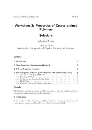
4.5 Chain with Excluded Volume InteractionsTask(4 points) Simulate a coarse-grained polymer with the same interactions and parameters as given above. In addition, apply Lennard-Jones interactions1to the monomers with 1, σ 1, and cutoff radius rc 2 6 . Shift theLennard-Jones function such that the force is zero for r rc . Repeat the simulations for the different values of N . Determine ν as in the previous task.SolutionNhRg 672Table 2: Radii of gyration hRg i of a self-avoiding chain for different chain lengths N simulated with ESPResSo 3.2.0. The average radii of gyration are listed in table 2. Fitting a function f (N ) aN ν to the simulation data yields an exponent ν 0.646, which is – as expected – greater than 0.5:self-avoiding chain simulationfit: 0.410N 0.646P (r)1050020406080100120140160180200rFigure 2: Radii of gyration hRg i of a self-avoiding chain for different chain lengths N simulated with ESPResSo 3.2.0.Dots ( ): Simulation data. Line (): fit.8

First, we rewrite equation (2) according to chapter 2.4 in Polymer Physics by Rubinstein: R2 g 1 N XN i 1 R i R com 2 1 N XN i 1 R 2 i 2R iR com R 2 com 1 N XN i 1 R 2 i 1 N XN j 1 1 2R i 1 N XN j 1 R j 1 N XN j 1 R j 2 1 N2 XN i 1 XN j 1 R 2 i 1 N2 N i 1 XN j 1 2R i R j 1 N XN i 1 1 N N j 1 R j 2 1 N2 XN i 1 N j 1 R 2 i 1 N2 N i 1 XN j 1 2R i R j 1 N2 N i 1 XN