Transcription
I.,ac.NASA-.-.A.CONTRACTORREPORTOI00P;U4cd4zLOAN COPY: RETURN TOAFWL (WLIL-2); iil%AND AFB, N MEXGUIDANCE,FLIGHTAND TRAJECTORYVolumeX - DynamicMECHANICSOPTIMIZATIONProgrammingby A. 5’. Abbott und J, E. McIntyrePreparedbyNORTH AMERICANDowney, Calif.for George C. MarshallAVIATION,Space FlightINC.CenterNATIONAL AERONAUTICSAND SPACEADMINISTRATION .WASHINGTON, D. C.APRIL 1968
TECH LIBRARY KAFB, NMllnllllllln lllnlllllClbflbb8NASA CR- 1009GUIDANCE,FLIGHTMECHANICSVolumeAND TRAJECTORYX - DynamicBy A. S. AbbottProgrammingand J. E. McIntyreDistributionof this report is providedResponsibilityinformationexchange.resides in the author or organizationIssuedby Originatoras Reportin the interest offor the contentsthat preparedit.No. SID 66-1678-2Prepared under Contract No. NAS 8-11495NORTH AMERICANAVIATION,INC.Downey, Calif.for GeorgeOPTIMIZATIONC. MarshallSpace FlightbyCenterNATIONAL AERONAUTICS AND SPACE ADMINISTRATIONFortk-.saleby 1Scientific- CFSTIand Technic01price 3.00- .Information
FOREWORDThis report was prepared under contract NAS 8-11495 and is one of a seriesintended to illustrateanalyticalmethods used in the fields of ight Mechanics, and TrajectoryBelow is a complete list of the reportsand recommended procedures are given.in the series.VolumeVolumeVolumeVolumeIIIIIIIVVolume VVolume oordinate Systems and Time MeasureObservation Theory and SensorsThe Two Body ProblemThe Calculus of Variationsand ModernApplicationsState Determinationand/or EstimationThe N-Body Problem and Special PerturbationTechniquesThe Pontryagin Maximum PrincipleBoost Guidance EquationsGeneral PerturbationsTheoryDynamic PrograrmningGuidance Equations for Orbital OperationsRelative Motion, Guidance Equations forTerminal RendezvousNumerical OptimizationMethodsEntry Guidance EquationsApplicationof OptimizationTechniquesMission Constraintsand TrajectoryInterfacesGuidance System Performance AnalysisThe work was conducted under the directionof C. D. Baker, J. W. Winch,and D. P. Chandler, Aero-Astro Dynamics Laboratory,George C. Marshall SpaceFlight Center., The North American program was conducted under the directionof H. A. McCarty and G. E. Townsend.iiic
TABIE OF CONTENTSSECTIONPAGE1.0STATEMENTOF THE PROBLEM. . . . . . . . . . . . . . . . . . .12.0STATE OF THE ART. . . . . . . . . . . . . . . . . . . . . . .32.12.22.32.4Development of Dynamic Programming .Fundamental Concepts and Applications.Simple Multi-StageDecision Problem. .2.2.12.2.2Simple Applicationsto Calculus of Variations.2.2.2.1Shortest Distance Problem .2.2.2.2VariationalProblem with aMovableBoundary. .2.2.2.3Simple Guidance Problem .Maximum Minimum Problem. .2.2.32.2.4Equipment Replacement Problem. .Computational Considerations.Merits of Dynamic Programming over2.3.1Conventional Analysis.2.3.1.1Relative Extrema. .2.3.1.2Constraints.2.3.1.3Continuity.Dynamic Programming versus Straightforward2.3.2CombinationalSearch .DifficultiesEncountered in Dynamic2.3.3Programming. .2.3.3.1Curse of Dimensionality.2.3.3.2Stabilityand Sensitivity.LimitingProcess in Dynamic Programming. .Recursive Equation for the Problem of Lagrange2.4.1Recursive Equation in LimitingForm. .2.4.2An Example Problem .2.4.3AdditionalPropertiesof the Optimal Solution.2.4.4Lagrange Problem with Variable End Points.2.4.5N-Dimensional Lagrange Problem .2.4.6Discussion of the Problem of Lagrange. .2.4.72.4.8The Problem of Bolza .Bellman Equation for the Bolza Problem .2.4.92.4.10Linear Problem with Quadratic Cost .2.4.11Dynamic Programming and the PontryaginMaximum Principle.2.4.12Some Limitationson the Development ofthe Bellman Equation 717578828792.98.10550
PAGESECTION2.5Dynamic Programming and the OptimizationofStochasticSystems. . . . . . . . . . . . . . . . . . . .108Introduction.Problem Statement .2.5.2.1PerfectlyObservable Case. .2.5.2.2PerfectlyInobservableCase. .2.5.2.3PartiallyObservable Case. .2.5.2.4Discussion.The Treatment of Terminal Constraints.2.5.3.1PerfectlyObservable Case. .2.5.3.2PerfectlyInobservableCase. .2.5.3.3PartiallyObservable Case. FERENCES.149'vi
1.0STATENI3JTOF THE PROBLENThis monograph will present both the theoreticaland computationalaspects of Dynamic Programming. The development of the subject matter inthe text will be similar to the manner in which Dynamic Programming itselfdeveloped. The first step in the presentation will be an explanation ofthe basic concepts of Dynamic Programming and how they apply to simplemulti-stagedecision processes. This effort will concentrate on the meaningof the principle of Optimality,optimal value functions, multistage decisionprocesses and other basic concepts.After the basic concepts are firmly in mind, the applicationsof thesetechniques to simple problems will be useful in acquiring the insight thatis necessary in order that the concepts may be applied to more complexproblems. The formulation of problems in such a manner that the techniquesof Dynamic Programming can be applied is not always simple and requiresexposure to many differenttypes of applicationsif this task is to bemastered. Further, the straightforwardDynamic Programming formulationis not sufficientto provide answers in some cases. Thus, many problemsrequire additionaltechniques in order to reduce computer core storageThe user is constantlyrequirements or to guarantee a stable solution.faced with trade-offsin accuracy, core storage requirements, and computationAll of these factors require insight that can only be gained from,thetime.examination of simple problems that specificallyillustrateeach of theseproblems.Since Dynamic Progrsmmin g is an optimizationtechnique, it is expectedthat it is related to Calculus of Variations and Pontryagin's MaximumSuch is the case. Indeed,.itPrinciple.is possible to derive the EulerLagrange equation of Calculus of Variations as well as the boundary conditionequations from the basic formulation of the concepts of Dynamic Programming.The solutions to both the problem of Lagrange and the problem of Mayer canalso be,derived from the Dynamic Programming formulation.In practice,however, the, theoreticalapplicationof the concepts of Dynamic Programmingpresent a differentapproach to some problems that are not easily formulatedby conventional techniques, and thus provides a powerful theoreticaltoolas well as a computational tool for optimizationproblems.The fields of stochastic and adaptive optimizationtheory have recentlyshown a new and challenging area of applicationfor Dynamic Programming.The recent applicationof the classical methods to this type of problem hasmotivated research to apply the concepts of Dynamic Programming with the hopethat insights and interpretationsafforded by these concepts will ultimatelyprove useful.1
2.02.1STATE OF THE ARTDevelopment of Dynamic ProgrammingThe mathematical formalism known as Wynsmic Programming" was developedby Richard Bellman during the early 1950's with one of the first accountsof the method given in the 1952 Proceedings of the Academy of Science(Reference 2.1.1).The name itselfappears to have been derived from therelated disciplineof Linear Programming, with the over-ridingfactor inthe selection of this name stemming more probably from the abundance ofresearch funding available for linear programming type problems, than fromthe limited technical similaritybetween the two.Dynamic Programmin g did not take long to become widely applied in manydifferenttypes of problems.In less than 15 years after its originationit has found its way into many differentbranches of science and is nowwidely used in the chemical, electricaland aerospace industries.However,even the most rapid perusal of any of Bellman's three books on the subject(Reference 2.1.2, 2.1.3, and 2.1.4) makes one point very clear:the fieldis notin which Dynamic Progr amming finds its most extensive applicationthat of science, but of economics, with the problems here all rather looselygroupable under the heading of getting the greatest amount of return fromthe least amount of investment.Of the several factors contributingtothis rapid growth and development, no small emphasis should be placed on thevigorous applicationprogram conducted by Bellman and his collegues at Randin which a multitude of problems were analyzed using the method, and theresults published in many differentJournals, both technical and non-technical.A brief biographicalsketch accompanying an article of Bellman's in a recentissue of the Saturday Review, (Ref. 2.1.5) states that his publicationsinclude 17 books and over 400 technical papers, a not-insignificantportionof which deal with the subject of Dynamic Programming.Historically,Dynamic Programming was developed to provide a means ofoptimizing multi-stagedecision processes. However, after this use wasfinallyestablished,the originatorsof Dynamic Programming began to usetheir mathematical licenses by considering practicallyall problems asmultistage decision processes.There were sound reasons behind such attempts.Firstj the solution of many practicalproblems by the use of,the classicalmethod of Calculus of Variations was extremely complicated and sometimesSecond, with the fields of high speed computers and mass dataimpossible.processing systems on the threshold, the idea of treating continuous systemsThis new breakin a multi-stage manner was very feasible and promising.through for Dynamic Progr amming gave rise to a study of the relationshipsbetween the Calculus of Variation and Dynamic Programming and applicationsto trajectoryprocesses and feedback control.3
The extension of Dynamic Programmin g to these other fields,however,presented computational problems.For example, it became necessary tostudy topics such as accuracy, stabilityand storage in order to handlethese more complicated problems. One of the beauties of Dynamic Programmingcame to rescue in solving some of these problems.It is idiosyncrasyexploitation.Whereas problem peculiaritiesusually are a burden to classicaltechniques, they are usually blessings to the dynamic programmer. It ispossible to save computation time, to save storage and/or to increase accuracyby exploitingproblem peculiaritiesin Dynamic Programming.An understanding of Dynamic Programming hinges on an understanding ofthe concept of a multi-stagedecision process, a concept which is mosteasily described by means of an example. Consider a skier at the top ofa hill who wishes to get down to the bottom of the hill as quickly aspossible.Assume that there are several trailsavailable which lead tothe bottom and that these trailsintersect and criss-crossone another asthe slope is descended. The down hill path which is taken will depend onlyon a sequence of decisions which the skier makes. The first decision consistsof selecting the trail on which to start the run. Each subsequent decisionis made whenever the current trail intersectssome new trail,at which pointthe skier must decide whether to take the new trail or not. Thus, associatedwith each set of decisions is a path leading to the bottom of the hill,andassociated with each path is a time, namely the time it takes to negotiatethe hill.The problem confronting the skier is that of selecting thatsequence of decisions (i.e.,the particularcombination of trails)whichresult in a minimum run time.From this example, it is clear that a multi-stagepossesses three important features:decisionprocess(1)To accomplish the objective of the process (in the examplea sequence ofabove, to reach the bottom of the hill)decisions must be made.(2)The decisions are coupled in the sense that the ntJ decision isaffected by all the prior decisions, and it, in turn, effectsIn the skier example, the veryall the subsequent decisions.existence of an n4fi decision depends on the preceding decisions.(3)Associated with each set of decisions there is a number whichdepends on all the decisions in the set (e.g., the time toThis number which goes by areach the bottom of the hill).variety of names will be referred to here as the performanceThe problem is to select that set of decisions whichindex.minimizes the performance index.
There are several ways to accomplish the specified objective and at thesame time minimize the performance index. The most direct approach wouldinvolve evaluating the performance index for every possible set of decisions.decision sets isHowever, in most decision processes the number of differentA secondso large that such an evaluation is computationallyimpossible.approach would be to endow the problem with a certain mathematical structuredifferentiability,analyticity,etc.), and then use a( e.g., continuity,standard mathematical technique to determine certain additional propertieswhich the optimal decision sequence must have. Two such mathematicaltechniques are the maxima-minima theory of the DifferentialCalculus andA third alternativeis to use Dynamic Programming.the Calculus of Variations.Dynamic Programming is essentiallya systematic search procedure forfinding the optimal decision sequence; in using the technique it is onlynecessary to evaluate the performance index associated with a small numberof all possible decision sets. This approach differs from the well-knownvariationalmethods, in that it is computational in nature and goes directlyto the determination of the optimal decision sequence without attempting touncover any special properties which this decision sequence might have. Inthis sense the restrictionson the problem's mathematical structure,whichare needed in the variationalapproach, are totallyunnecessary in DynamicProgramming. Furthermore, the inclusion of constraintsin the problem, asituation which invariablycomplicates a solution of the variationalmethods,facilitatessolution generation in the Dynamic Programming approach sincethe constraintsreduce the number of decision sets over which the searchmust be conducted.The physical basis for Dynamic Programming lies in the "Principle ofOptimality,"a principleso simple and so self -evident that one wouldhardly expect it could be of any importance.However, it is the recognitionof the utilityof this principlealong with its applicationto a broadspectrum of problems which constitutesBellman's major contribution.Besides its value as a computational tool, Dynamic Progr arming is alsoof considerable theoreticalimportance.If the problem possesses a certainmathematical structure,for example, if it is describable by a system ofdifferentialequations, then the additional properties of the optimaldecision sequence, as developed by the Maximum Principle or the Calculuscan also be developed using Dynamic Programming. This featureof Variations,gives a degree of completeness to the area of multi-stagedecision processesand allows the examination of problems from several points of view. Furthermore, there is a class of problems, namely stochastic decision processes,which appear to lie in the variationaldomain, and yet which escape analysisby means of the VariationalCalculus or the Maximum Principle.As will beshown, it is a rather straightforwardmatter to develop the additionalproperties of the optimal stochastic decision sequence by using DynamicProgramming.5
The purpose of this monograph is to present the methods of Dynamicits dual role as both a computational andProgrammin g and to illustratetheoreticaltool.In keeping with the objectives of the monograph series,the problems considered for solution will be primarilyof the trajectoryand control type arising in aerospace applications.It should be mentionedthat this particularclass of problems is not as well suited for solutionby means of Dynamic Programming as those in other areas. The systematicsearch procedure inherent in Dynamic Programming usually involves a verylarge number of calculationsoften in excess of the capabilityof presentcomputers. While this number can be brought within reasonable bounds,it is usually done at the expense of compromising solution accuracy.However, this situationshould change as both new methods and new computersare developed.The frequently excessive number of computations arising in trajectoryand control problems has somewhat dampened the initialenthusiasm with whichDynamic Programming was received.Many investigatorsfeel that theextensive applicationsof Dynamic Programming have been over-stated andthat computational procedures based upon the variationaltechniques are moresuitable for solution generation.However, it should be mentioned that theoriginatorsof these other procedures can not be accused of modesty whenit'comes to comparing the relative merits of their own technique with someThe difficultyarises in that each may be correct for certain classesother.of problems and unfortunately,there is littlewhich can be used to determinewhich will be best for a specific problem since the subject is relativelynewand requires much investigation.Without delineatingfurther the merits of Dynamic Programming in theintroductionit is noted that current efforts are directed to its applicationto more and more optimizationproblems. Since an optimizationproblem canalmost always be modified to a multi-stage decision processes, the extent ofapplicationof Dynamic Programming has encompassed business, military,managerial and technical problems. A partial list of applicationsappearsin Ref. 2.1.2.Some of the more pertinent fields are listed below.Allocation processesCalculus of VariationsCargo loadingCascade processesCommunication and InformationControl ProcessesEquipment ReplacementInventory and Stock LevelOptimal Trajectory ProblemsTheory6ProbabilityTheoryReliabilitySearch ProcessesSmoothingStochastic AllocationTransportationGame TheoryInvestment
2.2Fundamental Concepts and ApplicationsSection 2.1 presented the example of a skier who wishes to minimizethe time required to get to the bottom of the hill.It was mentioned thatthe Dynamic Programming solution to this problem resulted in a sequence ofdecisions, and that this sequence was determined by employing the Principleof Optimality.In this section, the Principle of Optimality and other basicconcepts will be examined in detail,and the applicationof these conceptswill be demonstrated on some elementary problems.The Principleof Optimalityis stated formallyin Ref. 0.4 as follows:An optimal policy has the property thatwhatever the initialstate and the initialdecisions are, the remaining decisions mustconstitutean optimal policy with regard tothe state resulting from the first decision.It is worthy to note that the Principle of Optimality can be statedmathematically as well as verbally.The mathematical treatment has beenplaced in section 2.4 in order that the more intuitiveaspects can bestressed without complicating the presentation.The reader interested inthe mathematical statement of the Principle is referred to Sections 2.4.1and 2.4.2Before this principlecan be applied, however, some measure of theperformance which is to be optimized must be established.This requirementintroduces the concept of the optimal value function.The optimal valuefunction is most easily understood as the relationshipbetween the parameterwhich will be optimized and the state of the process.In the case of theskier who wishes to minimize the time required to get to the bottom of thehill,the optimal value function is the minimum run time associated witheach intermediate point on the hill.Here the state of the process can bethought of as the location of the skier on the hill.The optimal valuefunction is referred to by many other names, depending upon the physicalnature of the problem. Some of the other names are t'cost function.""performance index," l'profit,"or "return function."However, whatever thename, it always refers to that variable of the problem that is to be optimized.Now that the concept of an optimal value function has been presented,the Principle of Optimality can be discussed more easily.In general, then stage multi-decisionprocess is the problem to which Dynamic Programmingis applied.However, it is usually a very difficultproblem to determinethe optimal decision sequence for the entire n stage process in one set ofcomputations.A much simplier problem is to find the optimum decision ofa one stage process and to employ Dynamic Programming to treat the n stageprocess as a series of one stage processes.This solution requires theinvestigationof the many one stage decisions that can be made from eachstate of the process.Although this procedure at first may appear as the7
"brute forcel' method (examining all the combinations of the possible decisions),it is the Principle of Optimality that saves this technique from the unwieldynumber of computations involved in the "brute force" method. This reasoningis most easily seen by examining a two stage process.Consider the problemof finding the optimal path from a point A to the LL' in the following sketch.The numbers on each line represent the "cost" of that particulartransition.This two stage process will now be treated as two one-stage processes.ThePrinciple of Optimality will then be used to determine the optimal decisionsequence. Starting at point A, the first decision to be made is whether toconnect point A to point B or point C. The Principle of Optimality states,however, that whichever decision is made the remaining choices must beoptimal.Hence, if the first decision is to connect A to B, then theremaining decision must be to connect B to E since it is the optimal pathfrom B to line LL'.Similarly,if the first decision is to connect A to C,then the remaining decision must be to connect C to E. These decisions enablean optimal cost to be associated with each of the points B and C; that is,the optimal cost from each of these points to the line LL'.Hence, theoptimal value of B is 5 and of C is 4 since these are the minimum costsfrom each of the points to line LL'.The first decision can be found by employing the Principle of Optimalityonce again. Now, however, the first decision is part of the remainingsequence, which must be optimal.The optimal value function must becalculated for each of the possibilitiesfor the first decision.If thefirst decis,ion is to go to B, the optimal value function at point A is thecost of that decision plus the optimal cost of the remaining decision, or,Similarly,the optimal value function at point A for a choice3 5 8.of C for the first decision is 2 4 6. Hence, the optimal first decisionis to go to C and the optimal second decision is to go to E. The optimalpath is thus, A-C-E.8
Although the previous problem was very simple in nature, it containsall the fundamental concepts involved in applying Dynamic Programming toa multi-stagedecision process. The remainder of this section uses thesame basic concepts and applies them to problems with a larger number ofstages and dimensions.9II.
2.2.1Multi-StageDecision ProblemThe basic ideas behind Dynamic Progr amming will now be applied to asimple travel problem. It is desired to travel from a certain city, A,to a second city, X, well removed from A.AXSince there are various types of travel services available to the minimum costfrom one intermediate city to another will vary depending upon the natureof the transportation.In general, this cost will not be strictlylinearwith distance.The intermediate cities-appearin the sketch above as theletters B, C, D, etc. with the cost in travelingbetween any two cities enteredon the connecting diagonal.The problem is to determine that route fortihich the total transportationcosts are a minimum. A similar problem istreated in Ref. 2.4.1.Obviously, one solution to this problem is to try all possible pathsfrom A to X, calculate the associated cost, and select the least expensive.Actually, for "small"problems this approach is not unrealistic.If, on theother hand, the problem is multi-dimensional,such a "brute force" methodis not feasible.First, consider the two ways of leaving city A. It is seen that theminimum cost of going to city B is 7, and city C is 5,. Based upon thisinformation a cost can be associated with each of the cities.Since thereare no less expensive ways of going from city A to these cities,the costassociated with each city is optimum. A table of costs can be constructedfor cities B and C as follows:10
Citgoptimum costB.A-BA-C75CPath for Optimum CostNow, the cost of cities D, E, and F will be found. The cost of D is 7 2 9.Since there are no other ways of getting to D, 9 is the optimum value.Thecost of city E,.on the other hand, is 13 by way of B and only 8 by way of C.So the optimum value of city E is 8. The cost for city F is 10 by way ofcity C. A table can now be constructed for cities D, E, and F as follows:CitsDEFOPthumcostBCC9810At this point, it is worthy to note two of the basic concepts that were used.Although they are very subtle in this case, they are keys to understandingDynamic Programming.First, the decision to find the cost of city E to be a minimum by choosingto go via city C is employing the Principle of Optimality.In this case, theoptimal value function, or cost, was optimized by making the current decisionsuch that all the previous decisions (including the recent one) yield anoptimum value at the present state.In other words, there was a choice ofgoing to city E via city B or C and city C was chosen because it optimizedthe optimal value function, which sums the cost of all previous decisions.One more stage will now be discussed so that the principlesare firmly inmind. Consider the optimum costs of cities G, H, I, and J. There is nochoice on the cost of city G. It is merely the optimum cost of city D (9)plus the cost of going to city G from city D ( 8), or 17. City H can bereached via city D or city E. In order to determine the optimum value forcity H, the optimum cost of city D plus the cost of travel from D to H iscompared to the optimum cost of E plus the cost of travel from E to H.In this case the cost via city E is 8 4 12 whereas the cost via D is9 14 23. Hence, the optimal value of city H is I2 and the optimum pathis via city E. By completely analogous computations the optimal-costandoptimum path for the remaining cities can be found and are shown below:Citgoptimum 1I,.
The previous computations are sufficientfor determining optimum path. Fromthe tables that have been constructed the optimum decision can be found.The following sketch shows the optimum decision for each point by an arrow.GThe optimum path, shown by a heavy line, can be found by starting at city Xand following the arrows to the left.It should be noted that the precedingcomputations were made from left to right,This constructionthen resultedin an optimum path which was determined from right to left.Identicalresultscould have been obtained if the computations are performed from right toleft.The following sketch shows the optimum decisions for this method ofattack.12
The optimum path can be found by starting at city A and following the arrowsfrom left to right.This path is shown by a heavy line in the sketch.There is an advantage to each of these computational procedures dependingupon the nature of the problem. In some problems, the terminal constraintsare of such a nature that it is computationallyadvantageous to start computingat the end of the problem and progress to the beginning.In other problems,the reverse may be true.The preceding sample problem was equally suitableto either method. Depending upon the formulation of the problem, the costsfor typical transitionsmay not be unique (the cost could depend upon thepath as in trajectoryproblems) as they were in the sample problem. Thismay be a factor that will influence the choice of the method to be used.To summarize, the optimal value function and the Principle of Optimalityhave been used to determine the best decision policy for the multi-stagedecision process: the optimal value function kept track of at least expensivepossible cost for each city while the Principle of Optimality used thisoptimum cost as a means by which it could make a decision for the nextstage of the process.Then, a new value for the optimal value function wascomputed for the next stage. After the computation was complete, each stagehad a corresponding decision that was made and which was used to determinethe optimum path.13
2.2.2Applicationsto the Calculus of VariationsSo far, the use of Dynamic Programmin g has been applied to multi-stagedecision processes.The same concepts can, however, be applied to thesolution of continuous variationalproblems providing the problem isformulated properly.As might be expected, the formulation involves adiscretizingprocess.The Dynamic Programming solution will be a discretizedversion of the continuous solution.Providing there are no irregularities,the discretizedsolution converges to the continuous solution in the limitas the increment is reduced in size.It is interestingto note that 'theformal mathematical statement of the concepts already introduced can beshown to be equivalent to the Euler-Lagrange equation in the Calculus ofVariations in the limit (see Section 2.4).The two classes of problemsthat are considered in this section are the problem of Lagrange and theand the problem of May
Flight Mechanics, and Trajectory Optimization. Derivations, mechanizations and recommended procedures are given. . Introduction. . 108 Problem Statement . 110 2.5.2.1 Perfectly Observable Case. . The solutions to both the problem of Lagrange and the problem of Mayer can also be,derived from the Dynamic Programming formulation. .