Transcription
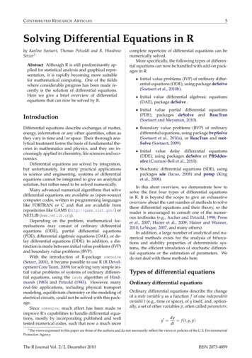
C ONTRIBUTED R ESEARCH A RTICLES5Solving Differential Equations in Rby Karline Soetaert, Thomas Petzoldt and R. WoodrowSetzer1Abstract Although R is still predominantly applied for statistical analysis and graphical representation, it is rapidly becoming more suitablefor mathematical computing. One of the fieldswhere considerable progress has been made recently is the solution of differential equations.Here we give a brief overview of differentialequations that can now be solved by R.IntroductionDifferential equations describe exchanges of matter,energy, information or any other quantities, often asthey vary in time and/or space. Their thorough analytical treatment forms the basis of fundamental theories in mathematics and physics, and they are increasingly applied in chemistry, life sciences and economics.Differential equations are solved by integration,but unfortunately, for many practical applicationsin science and engineering, systems of differentialequations cannot be integrated to give an analyticalsolution, but rather need to be solved numerically.Many advanced numerical algorithms that solvedifferential equations are available as (open-source)computer codes, written in programming languageslike FORTRAN or C and that are available fromrepositories like GAMS (http://gams.nist.gov/) orNETLIB (www.netlib.org).Depending on the problem, mathematical formalisations may consist of ordinary differentialequations (ODE), partial differential equations(PDE), differential algebraic equations (DAE), or delay differential equations (DDE). In addition, a distinction is made between initial value problems (IVP)and boundary value problems (BVP).With the introduction of R-package odesolve(Setzer, 2001), it became possible to use R (R Development Core Team, 2009) for solving very simple initial value problems of systems of ordinary differential equations, using the lsoda algorithm of Hindmarsh (1983) and Petzold (1983). However, manyreal-life applications, including physical transportmodeling, equilibrium chemistry or the modeling ofelectrical circuits, could not be solved with this package.Since odesolve, much effort has been made toimprove R’s capabilities to handle differential equations, mostly by incorporating published and welltested numerical codes, such that now a much morecomplete repertoire of differential equations can benumerically solved.More specifically, the following types of differential equations can now be handled with add-on packages in R: Initial value problems (IVP) of ordinary differential equations (ODE), using package deSolve(Soetaert et al., 2010b). Initial value differential algebraic equations(DAE), package deSolve . Initial value partial differential equations(PDE), packages deSolve and ReacTran(Soetaert and Meysman, 2010). Boundary value problems (BVP) of ordinarydifferential equations, using package bvpSolve(Soetaert et al., 2010a), or ReacTran and rootSolve (Soetaert, 2009). Initial value delay differential equations(DDE), using packages deSolve or PBSddesolve (Couture-Beil et al., 2010). Stochastic differential equations (SDE), usingpackages sde (Iacus, 2008) and pomp (Kinget al., 2008).In this short overview, we demonstrate how tosolve the first four types of differential equationsin R. It is beyond the scope to give an exhaustiveoverview about the vast number of methods to solvethese differential equations and their theory, so thereader is encouraged to consult one of the numerous textbooks (e.g., Ascher and Petzold, 1998; Presset al., 2007; Hairer et al., 2009; Hairer and Wanner,2010; LeVeque, 2007, and many others).In addition, a large number of analytical and numerical methods exists for the analysis of bifurcations and stability properties of deterministic systems, the efficient simulation of stochastic differential equations or the estimation of parameters. Wedo not deal with these methods here.Types of differential equationsOrdinary differential equationsOrdinary differential equations describe the changeof a state variable y as a function f of one independentvariable t (e.g., time or space), of y itself, and, optionally, a set of other variables p, often called parameters:y0 dy f (t, y, p)dt1 The views expressed in this paper are those of the authors and do not necessarily reflect the views or policies of the U.S. EnvironmentalProtection AgencyThe R Journal Vol. 2/2, December 2010ISSN 2073-4859
6In many cases, solving differential equations requires the introduction of extra conditions. In the following, we concentrate on the numerical treatmentof two classes of problems, namely initial value problems and boundary value problems.Initial value problemsIf the extra conditions are specified at the initial valueof the independent variable, the differential equations are called initial value problems (IVP).There exist two main classes of algorithms to numerically solve such problems, so-called Runge-Kuttaformulas and linear multistep formulas (Hairer et al.,2009; Hairer and Wanner, 2010). The latter containstwo important families, the Adams family and thebackward differentiation formulae (BDF).Another important distinction is between explicitand implicit methods, where the latter methods cansolve a particular class of equations (so-called “stiff”equations) where explicit methods have problemswith stability and efficiency. Stiffness occurs for instance if a problem has components with differentrates of variation according to the independent variable. Very often there will be a tradeoff between using explicit methods that require little work per integration step and implicit methods which are able totake larger integration steps, but need (much) morework for one step.In R, initial value problems can be solved withfunctions from package deSolve (Soetaert et al.,2010b), which implements many solvers from ODEPACK (Hindmarsh, 1983), the code vode (Brownet al., 1989), the differential algebraic equation solverdaspk (Brenan et al., 1996), all belonging to the linearmultistep methods, and comprising Adams methods as well as backward differentiation formulae.The former methods are explicit, the latter implicit.In addition, this package contains a de-novo implementation of a rather general Runge-Kutta solverbased on Dormand and Prince (1980); Prince andDormand (1981); Bogacki and Shampine (1989); Cashand Karp (1990) and using ideas from Butcher (1987)and Press et al. (2007). Finally, the implicit RungeKutta method radau (Hairer et al., 2009) has beenadded recently.Boundary value problemsIf the extra conditions are specified at differentvalues of the independent variable, the differential equations are called boundary value problems(BVP). A standard textbook on this subject is Ascheret al. (1995).Package bvpSolve (Soetaert et al., 2010a) implements three methods to solve boundary value problems. The simplest solution method is the singleshooting method, which combines initial value problem integration with a nonlinear root finding algoThe R Journal Vol. 2/2, December 2010C ONTRIBUTED R ESEARCH A RTICLESrithm (Press et al., 2007). Two more stable solution methods implement a mono implicit RungeKutta (MIRK) code, based on the FORTRAN codetwpbvpC (Cash and Mazzia, 2005), and the collocationmethod, based on the FORTRAN code colnew (Baderand Ascher, 1987). Some boundary value problemscan also be solved with functions from packages ReacTran and rootSolve (see below).Partial differential equationsIn contrast to ODEs where there is only one independent variable, partial differential equations (PDE)contain partial derivatives with respect to more thanone independent variable, for instance t (time) andx (a spatial dimension). To distinguish this typeof equations from ODEs, the derivatives are represented with the symbol, e.g. y y f (t, x, y, , p) t xPartial differential equations can be solved by subdividing one or more of the continuous independentvariables in a number of grid cells, and replacing thederivatives by discrete, algebraic approximate equations, so-called finite differences (cf. LeVeque, 2007;Hundsdorfer and Verwer, 2003).For time-varying cases, it is customary to discretise the spatial coordinate(s) only, while time is left incontinuous form. This is called the method-of-lines,and in this way, one PDE is translated into a largenumber of coupled ordinary differential equations,that can be solved with the usual initial value problem solvers (cf. Hamdi et al., 2007). This applies toparabolic PDEs such as the heat equation, and to hyperbolic PDEs such as the wave equation.For time-invariant problems, usually all independent variables are discretised, and the derivatives approximated by algebraic equations, which are solvedby root-finding techniques. This technique applies toelliptic PDEs.R-package ReacTran provides functions to generate finite differences on a structured grid. After that,the resulting time-varying cases can be solved withspecially-designed functions from package deSolve,while time-invariant cases can be solved with rootsolving methods from package rootSolve .Differential algebraic equationsDifferential-algebraic equations (DAE) contain amixture of differential ( f ) and algebraic equations(g), the latter e.g. for maintaining mass-balance conditions:y0 f (t, y, p)0 g(t, y, p)Important for the solution of a DAE is its index.The index of a DAE is the number of differentiationsISSN 2073-4859
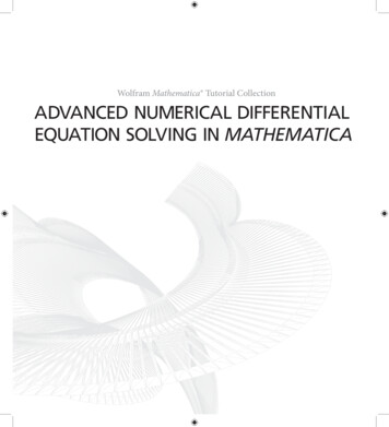
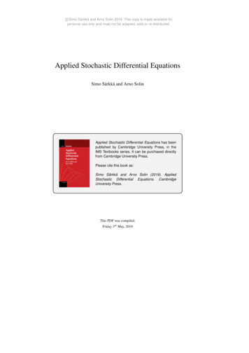
C ONTRIBUTED R ESEARCH A RTICLESneeded until a system consisting only of ODEs is obtained.Function daspk (Brenan et al., 1996) from package deSolve solves (relatively simple) DAEs of indexat most 1, while function radau (Hairer et al., 2009)solves DAEs of index up to 3.7Numerical accuracyNumerical solution of a system of differential equations is an approximation and therefore prone to numerical errors, originating from several sources:1. time step and accuracy order of the solver,2. floating point arithmetics,Implementation detailsThe implemented solver functions are explained bymeans of the ode-function, used for the solution ofinitial value problems. The interfaces to the othersolvers have an analogous definition:ode(y, times, func, parms, method c("lsoda","lsode", "lsodes", "lsodar","vode", "daspk", "euler", "rk4","ode23", "ode45", "radau", "bdf","bdf d", "adams", "impAdams","impAdams d"), .)To use this, the system of differential equationscan be defined as an R-function (func) that computesderivatives in the ODE system (the model definition)according to the independent variable (e.g. time t).func can also be a function in a dynamically loadedshared library (Soetaert et al., 2010c) and, in addition,some solvers support also the supply of an analytically derived function of partial derivatives (Jacobianmatrix).If func is an R-function, it must be defined as:func - function(t, y, parms, .)where t is the actual value of the independent variable (e.g. the current time point in the integration),y is the current estimate of the variables in the ODEsystem, parms is the parameter vector and . can beused to pass additional arguments to the function.The return value of func should be a list, whosefirst element is a vector containing the derivativesof y with respect to t, and whose next elements areoptional global values that can be recorded at eachpoint in times. The derivatives must be specified inthe same order as the state variables y.Depending on the algorithm specified in argument method, numerical simulation proceeds eitherexactly at the time steps specified in times, or using time steps that are independent from times andwhere the output is generated by interpolation. Withthe exception of method euler and several fixed-stepRunge-Kutta methods all algorithms have automatictime stepping, which can be controlled by setting accuracy requirements (see below) or by using optionalarguments like hini (initial time step), hmin (minimaltime step) and hmax (maximum time step). Specificdetails, e.g. about the applied interpolation methodscan be found in the manual pages and the originalliterature cited there.The R Journal Vol. 2/2, December 20103. properties of the differential system and stability of the solution algorithm.For methods with automatic stepsize selection,accuracy of the computation can be adjusted using the non-negative arguments atol (absolute tolerance) and rtol (relative tolerance), which controlthe local errors of the integration.Like R itself, all solvers use double-precisionfloating-point arithmetics according to IEEE Standard 754 (2008), which means that it can representnumbers between approx. 2.25 10 308 to approx. 1.8 10308 and with 16 significant digits. It is therefore not advisable to set rtol below 10 16 , except setting it to zero with the intention to use absolute tolerance exclusively.The solvers provided by the packages presentedbelow have proven to be quite robust in most practical cases, however users should always be awareabout the problems and limitations of numericalmethods and carefully check results for plausibility. The section “Troubleshooting” in the package vignette (Soetaert et al., 2010d) should be consulted asa first source for solving typical problems.ExamplesAn initial value ODEConsider the famous van der Pol equation (van derPol and van der Mark, 1927), that describes a nonconservative oscillator with non-linear damping andwhich was originally developed for electrical circuits employing vacuum tubes. The oscillation is described by means of a 2nd order ODE:z00 µ(1 z2 )z0 z 0Such a system can be routinely rewritten as a systemof two 1st order ODEs, if we substitute z00 with y10 andz0 with y2 :y10 y2y20 µ · (1 y1 2 ) · y2 y1There is one parameter, µ, and two differentialvariables, y1 and y2 with initial values (at t 0):y 1( t 0) 2y 2( t 0) 0ISSN 2073-4859
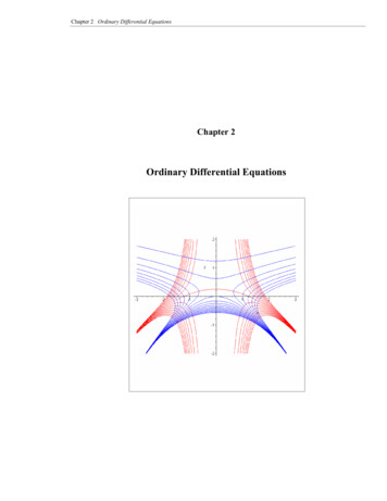
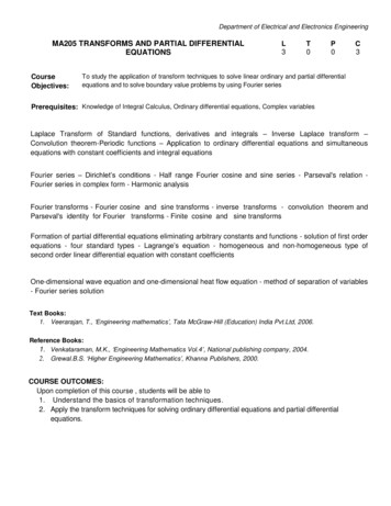
8 2 1012IVP ODE, stiffyThe van der Pol equation is often used as a testproblem for ODE solvers, as, for large µ, its dynamics consists of parts where the solution changesvery slowly, alternating with regions of very sharpchanges. This “stiffness” makes the equation quitechallenging to solve.In R, this model is implemented as a function(vdpol) whose inputs are the current time (t), the values of the state variables (y), and the parameters (mu);the function returns a list with as first element thederivatives, concatenated.C ONTRIBUTED R ESEARCH A RTICLES050010001500200025003000time 1012IVP ODE, nonstiff 2After defining the initial condition of the statevariables (yini), the model is solved, and outputwritten at selected time points (times), using deSolve’s integration function ode. The default routine lsoda, which is invoked by ode automaticallyswitches between stiff and non-stiff methods, depending on the problem (Petzold, 1983).We run the model for a typically stiff (mu 1000)and nonstiff (mu 1) situation:Figure 1: Solution of the van der Pol equation, aninitial value ordinary differential equation, stiff case,µ 1000.yvdpol - function (t, y, mu) {list(c(y[2],mu * (1 - y[1] 2) * y[2] - y[1]))}0library(deSolve)yini - c(y1 2, y2 0)stiff - ode(y yini, func vdpol,times 0:3000, parms 1000)nonstiff - ode(y yini, func vdpol,times seq(0, 30, by 0.01),parms 1)The model returns a matrix, of class deSolve,with in its first column the time values, followed bythe values of the state variables:head(stiff, n 3)51015202530timeFigure 2: Solution of the van der Pol equation, aninitial value ordinary differential equation, non-stiffcase, µ ]0 2.000000 0.0000000000[2,]1 1.999333 -0.0006670373[3,]2 1.998666 -0.0006674088Table 1: Comparison of solvers for a stiff and anon-stiff parametrisation of the van der Pol equation(time in seconds, mean values of ten simulations onan AMD AM2 X2 3000 CPU).Figures are generated using the S3 plot methodfor objects of class deSolve:A comparison of timings for two explicit solvers,the Runge-Kutta method (ode23) and the adamsmethod, with the implicit multistep solver (bdf,backward differentiation formula) shows a clear advantage for the latter in the stiff case (Figure 1). Thedefault solver (lsoda) is not necessarily the fastest,but shows robust behavior due to automatic stiffness detection. It uses the explicit multistep Adamsmethod for the non-stiff case and the BDF methodfor the stiff case. The accuracy is comparable for allplot(stiff, type "l", which "y1",lwd 2, ylab "y",main "IVP ODE, stiff")plot(nonstiff, type "l", which "y1",lwd 2, ylab "y",main "IVP ODE, nonstiff")The R Journal Vol. 2/2, December 2010ISSN 2073-4859
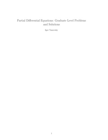
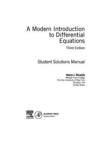
C ONTRIBUTED R ESEARCH A RTICLESsolvers with atol rtol 10 6 , the default.A boundary value ODEThe webpage of Jeff Cash (Cash, 2009) contains manytest cases, including their analytical solution (see below), that BVP solvers should be able to solve. Weuse equation no. 14 from this webpage as an example:ξy00 y (ξπ 2 1) cos(πx )on the interval [ 1, 1], and subject to the boundaryconditions:y( x 1) 0y( x 1) 0The second-order equation first is rewritten as twofirst-order equations:y10 y2y20 1/ξ · (y1 (ξπ 2 1) cos(πx ))9xi - 0.0025analytic - cos(pi * x) exp((x 1)/sqrt(xi)) exp(-(x 1)/sqrt(xi))max(abs(analytic - twp[, 2]))[1] 7.788209e-10A similar low discrepancy (4 · 10 11 ) is noted forthe ξ 0.0001 as solved by bvpcol; the shootingmethod is considerably less precise (1.4 · 10 5 ), although the same tolerance (atol 10 8 ) was usedfor all runs.The plot shows how the shape of the solutionis affected by the parameter ξ, becoming more andmore steep near the boundaries, and therefore moreand more difficult to solve, as ξ gets smaller.plot(shoot[, 1], shoot[, 2], type "l", lwd 2,ylim c(-1, 1), col "blue",xlab "x", ylab "y", main "BVP ODE")lines(twp[, 1], twp[, 2], col "red", lwd 2)lines(coll[, 1], coll[, 2], col "green", lwd 2)legend("topright", legend c("0.01", "0.0025","0.0001"), col c("blue", "red", "green"),title expression(xi), lwd 2)It is implemented in R as:BVP ODElibrary(bvpSolve)x - seq(-1, 1, by 0.01)shoot - bvpshoot(yini c(0, NA),yend c(0, NA), x x, parms 0.01,func Prob14)twp - bvptwp(yini c(0, NA), yend c(0,NA), x x, parms 0.0025,func Prob14)coll - bvpcol(yini c(0, NA),yend c(0, NA), x x, parms 1e-04,func Prob14)The numerical approximation generated by bvptwpis very close to the analytical solution, e.g. for ξ 0.0025:The R Journal Vol. 2/2, December 2010 1.0 0.50.00.50.010.00250.0001yWith decreasing values of ξ, this problem becomesincreasingly difficult to solve. We use three values of ξ, and solve the problem with the shooting,the MIRK and the collocation method (Ascher et al.,1995).Note how the initial conditions yini and the conditions at the end of the integration interval yendare specified, where NA denotes that the value is notknown. The independent variable is called x here(rather than times in ode).ξ1.0Prob14 - function(x, y, xi) {list(c(y[2],1/xi * (y[1] - (xi*pi*pi 1) * cos(pi*x))))} 1.0 0.50.00.51.0xFigure 3: Solution of the BVP ODE problem, for different values of parameter ξ.Differential algebraic equationsThe so called “Rober problem” describes an autocatalytic reaction (Robertson, 1966) between threechemical species, y1 , y2 and y3 . The problem can beformulated either as an ODE (Mazzia and Magherini,2008), or as a DAE:y10 0.04y1 104 y2 y3y20 0.04y1 104 y2 y3 3107 y221 y1 y2 y3ISSN 2073-4859
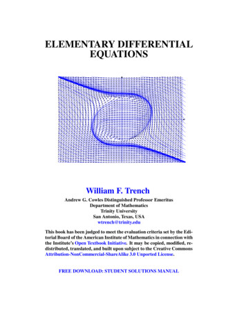
10C ONTRIBUTED R ESEARCH A RTICLESIVP DAEr2 y20 0.04y1 104 y2 y3 3 107 y22yini - c(y1 1, y2 0, y3 0)dyini - c(-0.04, 0.04, 0)times - 10 seq(-6,6,0.1)The input arguments of function daefun are thecurrent time (t), the values of the state variables andtheir derivatives (y, dy) and the parameters (parms).It returns the residuals, concatenated and an outputvariable, the error in the algebraic equation. The latter is added to check upon the accuracy of the results.For DAEs solved with daspk, both the state variables and their derivatives need to be initialised (yand dy). Here we make sure that the initial conditions for y obey the algebraic constraint, while alsothe initial condition of the derivatives is consistentwith the dynamics.library(deSolve)print(system.time(out -daspk(y yini,dy dyini, times times, res daefun,parms NULL)))user0.07system elapsed0.000.11An S3 plot method can be used to plot all variables at once:plot(out, ylab "conc.", xlab "time",type "l", lwd 2, log "x")mtext("IVP DAE", side 3, outer TRUE,line -1)There is a very fast initial change in concentrations, mainly due to the quick reaction between y1and y2 and amongst y2 . After that, the slow reactionof y1 with y2 causes the system to change much moresmoothly. This is typical for stiff problems.The R Journal Vol. 2/2, December 20101e 001e 061e 06timey3error1e 06conc. 5e 09 2e 090.80.40.0conc.1e 00time1e 09r3 1 y1 y2 y3Implemented in R this becomes:2e 05conc.0e 000.40.01e 06r1 y10 0.04y1 104 y2 y3daefun -function(t, y, dy, parms) {res1 - - dy[1] - 0.04 * y[1] 1e4 * y[2] * y[3]res2 - - dy[2] 0.04 * y[1] 1e4 * y[2] * y[3] - 3e7 * y[2] 2res3 - y[1] y[2] y[3] - 1list(c(res1, res2, res3),error as.vector(y[1] y[2] y[3]) - 1)}y20.8y1conc.where the first two equations are differentialequations that specify the dynamics of chemicalspecies y1 and y2 , while the third algebraic equationensures that the summed concentration of the threespecies remains 1.The DAE has to be specified by the residual function instead of the rates of change (as in ODEs).1e 061e 001e 061e 06time1e 001e 06timeFigure 4: Solution of the DAE problem for the substances y1 , y2 , y3 ; mass balance error: deviation of total sum from one.Partial differential equationsIn partial differential equations (PDE), the function has several independent variables (e.g. time anddepth) and contains their partial derivatives.Many partial differential equations can be solvedby numerical approximation (finite differencing) after rewriting them as a set of ODEs (see Schiesser,1991; LeVeque, 2007; Hundsdorfer and Verwer,2003).Functions tran.1D, tran.2D, and tran.3D fromR package ReacTran (Soetaert and Meysman, 2010)implement finite difference approximations of thediffusive-advective transport equation which, for the1-D case, is: 1 C ·Ax D · ( Ax · u · C)Ax x x xHere D is the “diffusion coefficient”, u is the “advection rate”, and A x is some property (e.g. surface area)that depends on the independent variable, x.It should be noted that the accuracy of the finitedifference approximations can not be specified in theReacTran functions. It is up to the user to make surethat the solutions are sufficiently accurate, e.g. by including more grid points.One dimensional PDEDiffusion-reaction models are a fundamental class ofmodels which describe how concentration of matter,energy, information, etc. evolves in space and timeunder the influence of diffusive transport and transformation (Soetaert and Herman, 2009).ISSN 2073-4859
C ONTRIBUTED R ESEARCH A RTICLESAs an example, consider the 1-D diffusionreaction model in [0, 10]: C C D· Q t x xwith C the concentration, t the time, x the distancefrom the origin, Q, the consumption rate, and withboundary conditions (values at the model edges):11user0.02system elapsed0.000.02The values of the state-variables (y) are plottedagainst the distance, in the middle of the grid cells(Grid x.mid).plot (Grid x.mid, std y, type "l",lwd 2, main "steady-state PDE",xlab "x", ylab "C", col "red") C 0 x x 0Cx 10 Cext20steady state PDEThe model equation includes a transport term,approximated by ReacTran function tran.1D anda consumption term (Q). The downstream boundary condition, prescribed as a concentration (C.down)needs to be specified, the zero-gradient at the upstream boundary is the default:pde1D -function(t, C, parms) {tran - tran.1D(C C, D D,C.down Cext, dx Grid) dClist(tran - Q) # return value: rate of change}The model parameters are: 10 30library(ReacTran)Grid - setup.grid.1D(N 1000, L 10)C010To solve this model in R, first the 1-D model Grid isdefined; it divides 10 cm (L) into 1000 boxes (N).0246810xFigure 5: Steady-state solution of the 1-D diffusionreaction model.The analytical solution compares well with thenumerical approximation:analytical - Q/2/D*(Grid x.mid 2 - 10 2) Cextmax(abs(analytical - std y))[1] 1.250003e-05D - 1Q - 1Cext - 20# diffusion constant# uptake rateIn a first application, the model is solved tosteady-state, which retrieves the condition where theconcentrations are invariant: C0 D· Q x xIn R, steady-state conditions can be estimated usingfunctions from package rootSolve which implementamongst others a Newton-Raphson algorithm (Presset al., 2007). For 1-dimensional models, steady.1D ismost efficient. The initial “guess” of the steady-statesolution (y) is unimportant; here we take simply Nrandom numbers. Argument nspec 1 informs thesolver that only one component is described.Although a system of 1000 equations needs to besolved, this takes only a fraction of a second:Next the model is run dynamically for 100 timeunits using deSolve function ode.1D, and startingwith a uniform concentration:require(deSolve)times - seq(0, 100, by 1)system.time(out - ode.1D(y rep(1, Grid N),times times, func pde1D,parms NULL, nspec 1))user0.61system elapsed0.020.63Here, out is a matrix, whose 1st column containsthe output times, and the next columns the values ofthe state variables in the different boxes; we print thefirst columns of the last three rows of this matrix:tail(out[, 1:4], n 3)library(rootSolve)print(system.time(std - steady.1D(y runif(Grid N),func pde1D, parms NULL, nspec 1)))The R Journal Vol. 2/2, December 2010[99,][100,][101,]time12398 -27.55783 -27.55773 -27.5575499 -27.61735 -27.61725 -27.61706100 -27.67542 -27.67532 -27.67513ISSN 2073-4859
12C ONTRIBUTED R ESEARCH A RTICLESWe plot the result using a blue-yellow-red colorscheme, and using deSolve’s S3 method image. Figure 6 shows that, as time proceeds, gradients developfrom the uniform distribution, until the system almost reaches steady-state at the end of the simulation.image(out, xlab "time, days",ylab "Distance, cm",main "PDE", add.contour TRUE)1.0PDE15100.850Distance, cm0.6 5 100.4 15 200.00.2 25020406080100time, daysFigure 6: Dynamic solution of the 1-D diffusionreaction model.It should be noted that the steady-state model iseffectively a boundary value problem, while the transient model is a prototype of a “parabolic” partial differential equation (LeVeque, 2007).Whereas R can also solve the other two mainclasses of PDEs, i.e. of the “hyperbolic” and “elliptic” type, it is well beyond the scope of this paper toelaborate on that.DiscussionAlthough R is still predominantly applied for statistical analysis and graphical representation, it is moreand more suitable for mathematical computing, e.g.in the field of matrix algebra (Bates and Maechler,2008). Thanks to the differential equation solvers, Ris also emerging as a powerful environment for dynamic simulations (Petzoldt, 2003; Soetaert and Herman, 2009; Stevens, 2009).The new package deSolve has retained all thefuntionalities of its predecessor odesolve (Setzer,2001), such as the potential to define models both inR code, or in compiled languages. However, compared to odesolve, it includes a more complete setof integrators, and a more extensive set of options totune the integration routines, it provides more complete output, and has extended the applicability domain to include also DDEs, DAEs and PDEs.Thanks to the DAE solvers daspk (Brenan et al.,1996) and radau (Hairer and Wanner, 2010) it is nowalso possible to model electronic circuits or equilibrium chemical systems. These problems are often ofindex 1. In many mechanical systems, physicalconstraints lead to DAEs of index up to 3, and thesemore complex problems can be solved with radau.The inclusion of BVP and PDE solvers haveopened up the application area to the field of reactive transport modelling (Soetaert and Meysman,2010), such that R can now be used to describe quantities that change not only in time, but also alongone or more spatial axes. We use it to model howecosystems change along rivers, or in sediments, butit could equally serve to model the growth of a tumor in human brains, or the dispersion of toxicantsin human tissues.The open source matrix language R has great potential for dynamic modelling, and the tools currently available are suitable for solving a wide variety of practical and scientific problems. The performance is sufficient even for larger systems, especiallywhen models can be formulated using matrix algebra or are implemented in compiled languages likeC or Fortran (Soetaert et al., 2010b). Indeed, thereis emerging interest in performing statistical analysison differential equations, e.g. in package nlmeODE(Tornøe et al., 2004) for fitting non-linear mixedeffects models using differential equations, package FME (Soetaert and Petzoldt, 2010) for sensitivity analysis, parameter estimation and Markov chainMonte-Carlo analysis or package ccems for combinatorially complex equilibrium model selection (Radivoyevitch, 2008).However, there is ample room for extensionsand improvements. For instance, the PDE solversare quite memory intensive, and could benefit fromthe implementation of sparse matrix solvers that aremore efficient in this respect2 . In addition, the methods implemented in ReacTran handle equations defined on very simple shapes only. Extending thePDE approach to finite elements (Strang and Fix,1973) would open up the application domain of R toany irregular geometry. Other spatial discretisationschemes could be added, e.g. for use in fluid dynamics.Our models are often applied to derive unknownparameters by fitting them against data; th
plied for statistical analysis and graphical repre-sentation, it is rapidly becoming more suitable for mathematical computing. One of the fields where considerable progress has been made re-cently is the solution of differential equations. Here we give a brief overview of differential equations that can now be solved by R. Introduction