Transcription
A Large Contextual Dataset for Classification,Detection and Countingof Cars with Deep LearningT. Nathan Mundhenk(B) , Goran Konjevod,Wesam A. Sakla, and Kofi BoakyeComputational Engineering Division,Lawrence Livermore National Laboratory, Livermore, gmail.comAbstract. We have created a large diverse set of cars from overheadimages (Data sets, annotations, networks and scripts are available fromhttp://gdo-datasci.ucllnl.org/cowc/), which are useful for training a deeplearner to binary classify, detect and count them. The dataset and allrelated material will be made publically available. The set contains contextual matter to aid in identification of difficult targets. We demonstrateclassification and detection on this dataset using a neural network we callResCeption. This network combines residual learning with Inceptionstyle layers and is used to count cars in one look. This is a new wayto count objects rather than by localization or density estimation. It isfairly accurate, fast and easy to implement. Additionally, the countingmethod is not car or scene specific. It would be easy to train this methodto count other kinds of objects and counting over new scenes requires noextra set up or assumptions about object locations.Keywords: Deep · Learning · CNNAutomobile · Classification · Detection1· COWC ·· CountingContext·Cars·IntroductionAutomated analytics involving detection, tracking and counting of automobilesfrom satellite or aerial platform are useful for both commercial and governmentpurposes. For instance, [1] have developed a product to count cars in parking lotsfor investment customers who wish to monitor the business volume of retailers.Governments can also use tracking and counting data to monitor volume and pattern of traffic as well as volume of parking. If satellite data is cheap and plentifulenough, then it can be more cost effective than embedding sensors in the road.A problem encountered when trying to create automated systems for thesepurposes is a lack of large standardized public datasets. For instance OIRDS [2]has only 180 unique cars. A newer set VEDAI [3] has 2950 cars. However, bothof these datasets are limited by not only the number of unique objects, but theyc Springer International Publishing AG 2016 B. Leibe et al. (Eds.): ECCV 2016, Part III, LNCS 9907, pp. 785–800, 2016.DOI: 10.1007/978-3-319-46487-9 48
786T.N. Mundhenk et al.also tend to cover the same region or use the same sensors. For instance, allimages in the VEDAI set come from the AGRC Utah image collection [4].We have created a new large dataset of Cars Overhead with Context (COWC).Our set contains a large number of unique cars (32,716) from six different imagesets each covering a different geographical location and produced by differentimagers. The images cover regions from Toronto Canada [5], Selwyn New Zealand[6], Potsdam [7] and Vaihingen Germany [8], Columbus [9] and Utah [4] UnitedStates. The set is also designed to be difficult. It contains 58,247 usable negativetargets. Many of these have been hand picked from items easy to mistake forcars. Examples of these are boats, trailers, bushes and A/C units. To compensatefor the added difficulty, context is included around targets. Context can help tellus something may not be a car (is sitting in a pond?) or confirm it is a car(between other cars, on a road). In general, the idea is to allow a deep learnerto determine the weight between context and appearance such that somethingthat looks very much like a car is detected even if it’s in an unusual place.2Related WorkWe will focus on three tasks with our data set. The first task is a two-classclassifier. To some extent, this is becoming trivial. For instance, [10] reports near100 % classification on their set. This is part of the reason for trying to increasethe difficulty of targets. Our contribution in this task is to demonstrate goodclassification on an intentionally difficult dataset. Also, we show that contextdoes help with this task, but probably mostly on special difficult cases.A more difficult problem is detection and localization. A very large number ofdetectors start with a trained classifier and some method for testing spatial locations to determine if a target is present. Many approaches use less contemporarySVM and Boosting based methods, but apply contextual assistance such as roadpatch detection or motion to reduce false positives [3,11–13]. Some methods usea deep learning network with strided locations [1,10] that generate a heat map.Our method for detection is similar to these, but we include context by expanding the region to be inspected in each stride. We also use a more recent neuralnetwork which can in theory handle said context better.By far our most interesting contribution that uses our new data set is vehiclecounting. Most contemporary counting methods can be broadly categorized asa density estimator [14–16] or, detection instance counter [11,13,17]. Densityestimators try to create an estimation of the density of a countable object andthen integrate over that density. They tend not to require many training samples,but are usually constrained to the same scene on which it was trained. Detectioncounters work in the more intuitive fashion of localizing each car uniquely andthen counting the localizations. This can have the downside that the entire imageneeds to be inspected pixel by pixel to create the localizations. Also, occlusionsand overlapping objects can create a special challenge since a detector may mergeoverlapping objects. Another approach tries to count large crowds of people bytaking a fusion over many kinds of feature counts using a Markov random field
Classification, Detection and Counting of Cars with Deep Learning787constraint [18] and seems like a synthesis of the density and detection approaches.However, it uses object-specific localizers such as a head detector so it is unclearhow well it would generalize to other objects.Our method uses another approach. We teach a deep learning neural networkto recognize the number of cars in an extended patch. It is trained only to countthe number of objects as a class and is not given information about locationor expected features. Then we count all the cars in a scene using a very largestride by counting them in groups at each stride location. This allows us totake one look at a large location and count by appearance. It has recently beendemonstrated that one-look methods can excel at both speed and accuracy [19]for recognition and localization. The idea of using a one-look network counter tolearn to count has recently been demonstrated on synthetic data patches [20] andby regression on subsampled crowd patches [21]. Here we utilize a more robustnetwork, and demonstrate that a large strided scan can be used to quickly counta very large scene with reasonable accuracy. Additionally, we are not constrainedby scene or location. Cars can be automatically counted anywhere in the world,even if they are not on roads or moving.3Data Set DetailsOverhead imagery from the six sources is standardized to 15 cm per pixel atground level from their original resolutions. This makes cars range in size from24 to 48 pixels. Two of the sets (Vaihingen, Columbus) are grayscale. The otherfour are in RGB color. Typically, we can determine the approximate scale atground level from imagery in the field (given metadata from camera and GPS,IMU calibrated SFM [22] or a priori known position for satellites). So we donot need to deal with scale invariance. However, we cannot assume as much interms of quality, appearance or rotation. Many sets can still be in grayscale orhave a variety of artifacts. Most of our data have some sort of orthorectificationartifacts in places. These are common enough in most overhead data sets thatthey should be addressed here.The image set is annotated by single pixel points. All cars in the annotatedimages have a dot placed on their center. Cars that have occlusions are includedso long as the annotator is reasonably sure the item is a car. Large trucks arecompletely omitted since it can be unclear when something stops being a lightvehicle and starts to become a truck. Vans and pickups are included as cars evenif they are large. All boats, trailers and construction vehicles are always addedas negatives. Each annotated image is methodically searched for any item thatmight at least slightly look like a car. These are then added. It is critical to tryand include as many possible confounders as we can. If we do not, a trainedsystem will underperform when introduced to new data.Occasionally, some cars are highly ambiguous or may be distorted in theoriginal image. Whether to include these in the patch sets depends on the task.For the classification task, if it was unclear if an item was or was not a car, it wasleft out. Distorted cars were included so long as the distortion was not too grave.
788T.N. Mundhenk et al.In both cases, this is a judgment call. For the counting task, one is forced to dealwith these items since they appear incidentally in many training patches. Forthat, a best guess is made. If a car was highly distorted, it was counted as a carso long as it appeared to be a car.To extract training and testing patches from large overhead images, theywere subdivided into grids of size 1024 1024 (see Fig. 1). These grid regionswere automatically assigned as training or testing regions. This keeps trainingand testing patches separate. The two types of patches cannot overlap. However, testing image patches may overlap other testing image patches and training patches overlap other training patches. In places like crowded parking lots,patches necessarily overlap. Every fourth grid location was used for testing. Thiscreates an approximate ratio of more than three training patches for each testingpatch. The patches are extracted in slightly different ways for different tasks. Wedo not include a validation set because we use a held out set of 2048 2048 sceneimages for final testing in the wild for each given task.Fig. 1. The locations from which testing and training patches were extracted from anoverhead image of Toronto. Blue areas are training patch areas while red areas aretesting patch areas. (Color figure online)Each held out scene is 2048 2048 (see Fig. 2). This is approximately 307 307meters in size at ground level. Held out scenes are designed to be varied andnon-trivial. For instance, one contains an auto reclamation junkyard filled withbanged up cars. We have 10 labeled held out scene images, and 10 more wherecars have been counted but not labeled. An additional 2048 2048 validationscene was used to adjust parameters before running on the held out scene data.The held out data is taken from the Utah set since there is an abundance offree data. They are also taken from locations far from where the patch data wastaken. Essentially, all patch data was taken from Salt Lake City and all held outdata was taken from outside of that metropolitan area. The held out data alsocontains mountainous wooded areas and a water park not found anywhere in thepatch data. Other unique areas such as the aforementioned auto junkyard anda utility plant are included, but there are analogs to these in the patch data.
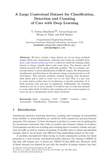
Classification, Detection and Counting of Cars with Deep Learning789Fig. 2. Three examples of 2048 2048 held out scenes we used. These include a mixedcommercial industrial area, a water park and a mountain forest area.4Classification and DetectionWe created a contextual set of patches for classification training. These are sized256 256. We created rotational variants with 15 degree aligned offsets of eachunique car and each unique negative. This yielded a set of 308,988 trainingpatches and 79,447 testing patches. A patch was considered to contain a carif it appeared in a central 48 48 region (The largest expected car length).Any car outside this central region was considered context. So, negative patchesfrequently had cars in them, so long as the car did not fall inside the 48 48pixel region. An edge margin of 32 pixels was grayed out in each patch. This wasdetermined to provide the optimal context (see Sect. 4.1 “Does Context Help?”).Fig. 3. left A standard Inception layer. right A ResCeption layer. The primary difference between it and Inception is that the 1 1 convolutions are used as a residualshortcut with projection.We trained a few different networks for comparison. Since we want to includecontextual information, larger more state-of-the-art networks are used. Weused AlexNet [23] as our smaller baseline and GoogLeNet/Inception with batchnormalization [24,25]. We created a third network to synthesize Residual Learning [26] with Inception. We called this one ResCeption (Fig. 3). The ResCeption
790T.N. Mundhenk et al.network is created by removing the 1 1 convolutions in each Inception layer andreplacing them with a residual “projection shortcut”. In section five, the advantage of doing this will become more apparent. [27] published to arXiv at the timeof this writing, is similar, but keeps the 1 1 convolution layers. These seemredundant with the residual shortcut which is why we removed them. The ResCeption version of GoogLeNet has about 5 % more operations than the Inceptionversion, but interestingly runs about 5 % faster on our benchmark machine. Allthree networks were trained using Caffe [28] and stochastic gradient descent for240 k iterations with a mini batch size of 64. A polynomial rate decay policy wasused with initial learning rate of 0.01 and power of 0.5. Momentum was 0.9 andweight decay 0.0002. The network input size was 224 224, so training imageswere randomly cropped to move the target a little around inside the 48 48central region. Testing images were center-cropped.Table 1. The percentage of test patches correctly classified for each deep model. TheNon-Utah model was trained with non-Utah data (the other five sets) and then testedwith Utah data to observe generalization to new datasets.ModelCorrectAlexNet97.62 %Inception99.12 %ResCeption99.14 %ResCeption non-utah 98.89 %Table 1 shows that Inception and ResCeption work noticeably better thanAlexNet. However, all three seem to do pretty well. Figure 4 shows examples ofpatches the ResCeption network got correct.4.1Does Context Help?We were interested to determining if context really helps classification results.To do this, we created sets where we masked out margins of the patches. Byadjusting the size of the margin, we can determine performance changes as moreor less of each patch is visible. We did this in increments of 32 pixels startingfrom the smallest possible region with only 32 32 pixels visible. Each trainingwas done on GoogLeNet by fine-tuning the default version from Caffe. Figure 5shows the results. Even the version with a small amount of context does well,but performance does increase monotonically until 192 192 pixels are visible.This suggests that most of the time, context is not all that important. Cars seemeasy to classify. Context might only help in the 1 % or 2 % of difficult cases wherestrong occlusions and poor visibility make a determination difficult. That we canhave too much context might be a result of too much irrelevant information orbad hints from objects that are too far from a car.
Classification, Detection and Counting of Cars with Deep Learning791Fig. 4. (top row) Test patches which the ResCeption network correctly classified ascontaining a car in the central region. Occlusions and visibility issues are commonlyhandled, but we note that they still appear to account for much of the error. (bottomrow) Patches that were correctly classified as not containing a car in the central region.The leftmost image is not a mistake. It has a tree in the center while the shifted versionabove it has a car concealed slightly underneath the tree.4.2DetectionNext we wanted to ascertain how well our trained network might perform ona real world task. One task of interest, is target verification. In this, anotheritem such an object tracker [29] would have been assigned to track a target car.Our network would then be used to verify each frame to tell if the tracker wasstill tracking a car or if it had drifted to another target. A second more difficulttask would involve localization and detection. This is the ability to find cars anddetermine where they are in a natural scene. The two tasks are almost equivalentin how we will test them. The biggest difference is how we score the results.For this task we used the trained ResCeption network since it had a slightlybetter result than Inception. Each of the 10 labeled 2048 2048 scene imagewere scanned with a stride of eight. At each stride location, 192 192 pixelswere extracted and a 32 pixel margin was added to create a 224 224 patch.Fig. 5. The percentage of correct patches versus the amount of context present. Asmore context is included, accuracy improves. It appears optimal to cut out a smallamount of context.
792T.N. Mundhenk et al.The softmax output was computed and taken to the power of 16 to create awider gradient for the output around the extremes:p (o1 o2 1)16/216(1)Fig. 6. (left) A held out scene super imposed with the derived heat map colored inred. (right) A close up of one of the sections (highlighted in yellow on left) showingexamples of detections and misses. The lower left car is considered detected since it ismostly inside the box. The false positive appears to be a shed. (Color figure online)This yielded a heat map with pixels p created from softmax outputs car o1 andnot car o2 . The value ranged from 0 to 1 with a strong upper skew. Location wasdetermined using basic non-maximal suppression on the heat map (keeping itsimple to establish a baseline). Bounding boxes were fixed at size 48 pixels whichis the maximum length of a car. Boxes could overlap by as much as 20 pixels.Maximal locations were thresholded at 0.75 to avoid weak detections. Thesevalues were established on a special validation scene, not the hold out scenes.A car was labeled as a detection if at least half of its area was inside a boundingbox. A car was a false negative if it was not at least half inside a box. A falsepositive occurred when a bounding box did not have at least half a car inside it.For the verification condition, splits (two or more detections on the same car)and mergers (two or more cars only covered by one box) did not count sincethese are not an effect that should impact its performance. For detection, a splityielded an extra false positive per extraneous detection. A merger was countedas a false negative for each extra undetected car. Figure 6 shows examples ofdetections from our method.In Table 2, we can see the results for both conditions. Typically for car detections without explicit location constraints, precision/recall statistics range from75 % to 85 % [3,10] but may reach 91 % if the problem is explicitly constrained tocars on pavement only [11–13]. This is not an exact comparison, but an F-scoreof 94.37 % over an unconstrained area of approximately 1 km2 suggests we aredoing relatively well.
Classification, Detection and Counting of Cars with Deep Learning793Table 2. Verification and detection performance is shown for the ResCeption model.Count is the number of cars in the whole set. TP, FP and FN are true positive, falsepositive and false negative counts. F is the precision/recall related F-Score. Ideally theverification score should be similar to the patch correctness which was 99.14 %. So, wedo incur some extra error. Detection error is higher since it includes splits and mergers.Condition5Count TP FP FN Precision RecallFVerification 2602539796.56 %97.31 % 96.93 %Detection250 201092.59 %96.15 % 94.34 %260CountingThe goal here was to create a one-look [19] counting network that would learn thecombinatorial properties of cars in a scene. This is an idea that was previouslydescribed in [20] who counted objects in synthetic MNIST [30] scenes using asmaller five-layer network. The overhead scenes we wish to count from are toolarge for a single look since they can potentially span trillions of pixels. However,we may be able to use a very large stride and count large patches at a time. Thus,the counting task is broken into two parts. The first part is learning to countby one-look over a large patch. The second part is creating a stride that countsobjects in a scene one patch at a time.Training patches are sampled the same as for the classification task. However,the class for each patch is the number of cars in that patch. Very frequently, carsare split in half at the border of the patch. These cars are counted if the pointannotation is at least 8 pixels into the visible region of the image. Thus, a carmust be mostly in the patch in order to be counted. If a highly ambiguous objectwas in a patch, we did our best to determine whether it was or was not a car.This is different from the classification task were ambiguous objects could beleft out. Here, they were too common as member objects that would incidentallyappear in a patch even if not labeled.We trained AlexNet [23], Inception [24,25] and ResCeption networks whichonly differed from the classification problem in the number of outputs. Here, weused a softmax with 64 outputs. A regression output may also be reasonable,but the maximum number of cars in a scene is sufficiently small that a softmaxis feasible. Also, we cover the entire countable interval. So there are no gaps thatwould necessitate using regression. In all the training patches, we never observedmore than 61 cars. We rounded up to 64 in case we ever came upon a set thatlarge and wanted to fine tune over it.We also trained a few new networks. The main idea for creating the ResCeption network was to allow us to stack Inception like layers much higher.This could give us the lightweight properties of GoogLeNet, but the ability togo big like with ResNet [26]. Here we have created a double tall GoogLeNet likenetwork. This is done by repeating each ResCeption layer twice giving us 22 ResCeption layers rather than 11. It was unclear if we needed three error outputs
794T.N. Mundhenk et al.like GoogLeNet, so we created two versions of our taller network. One doubletall network has only one error output (o1) while another has three in the samefashion as GoogLeNet (o3).Fig. 7. Examples of patches which were correctly counted by the ResCeption Tallero3 network. From left to right the correct number is 9, 3, 6, 13 and 47. Note that carswhich are not mostly inside a patch are not counted. The center of the car must be atleast 8 pixels inside the visible region.For the non-tall networks, training parameters were the same as with classification. For the double tall networks, the mini batch size was reduced to 43to fit in memory and the training was extended to 360 k iterations so that thesame number of training exposures are used for both tall and non-tall networks.Table 3 shows the results of error in counting on patch data. Examples of correctpatch counts can be seen in Fig. 7. It’s interesting to note that we can train avery tall GoogLeNet like network with only one error output. This suggests thatthe residual component is doing its job.Table 3. The patch based counting error statistics. The first data column is the percentage of test patches the network gets exactly correct. The next two columns showthe percentage counted within 1 or 2 cars. MAE is the mean absolute error of count.RMSE is the root mean square error. The last column is the accuracy if we used thecounting network as a proposal method. Thus, if we count zero cars, the region wouldbe proposed to contain no cars. If the region contains at least one car, we proposethat region has at least one car. The Taller ResCeption network with just one erroroutput has the best metrics in three of the six columns. However, the improvement issomewhat modest.ModelCorrect is / 1 is / 2 MAE RMSE Proposal AccAlexNet67.97 % 95.69 %98.82 %0.5271.19295.32 %Inception80.35 % 95.89 %98.87 %0.2570.66597.79 %ResCeption80.34 % 95.95 %98.86 %0.2550.657 97.69 %ResCeption taller o1 81.07% 96.11 % 98.89 %ResCeption taller o3 80.82 % 96.08 %0.248 0.67698.95 % 0.2500.66597.84 %97.83 %
Classification, Detection and Counting of Cars with Deep Learning5.1795Counting ScenesOne of the primary difficulties in moving from counting cars in patches to counting cars in a scene using a large stride is that if we do not have overlap betweenstrides, cars may be cut in half and counted twice or not at all. Since cars haveto be mostly inside a patch, some overlap would be ideal. Thus, by requiringthat cars are mostly inside the patch, we have created a remedy to the splittingand counting twice problem, but have increased the likelihood of not countinga split car at all. In this case, since we never mark the location of cars, thereis no perfect solution for this source of error. We cannot eliminate cars as wecount because we do not localize them. However, we can adjust the stride tominimize the likelihood of this error. We used the special validation scene with628 cars and adjusted the stride until error was as low as possible. This resultedin a stride of 167. We would then use this stride in any other counting scene.An example of a strided count can be seen in Fig. 8. To allow any stride andmake sure each section was counted, we padded the scene with zeros so that thecenter of the first patch starts at (0,0) in the image.Fig. 8. A subsection of one of the held out scenes. It shows the stride used by thenetwork as well as the number of cars it counted in each stride. Blue and green bordersare used to help differentiate the region for each stride. One can see the overlappingregion where the strides cross. 74 cars are counted among the six strides seen. Thesub-scene contains 77 complete cars. Note that cars on their side are not counted sincewe are only concerned with cars that are mobile. (Color figure online)We tested counting on a held out set of 20 2048 2048 scenes. The number ofcars in each scene varied between 881 and 10 with a mean of 173. Each held outscene was from the Utah AGRC image set. However, we selected geolocationswhich were unique. All Utah patch data came from the Salt Lake City metropolitan area. The held out data came from locations outside of that metro. Theseincluded some unusual and difficult locations such as mountain forest, a waterpark and an auto junkyard. Many of the scenes have dense parking lots, but
796T.N. Mundhenk et al.many do not. We included industrial, commercial and residential zones of different densities. The error results can be seen in Table 4. It is interesting to notethat while the double tall ResCeption network with one output dominates thepatch results, the double tall ResCeption network with three outputs dominatesthe scene results. This may be related to the lower RMSE and / 2 error forthe three-output network. The network may be less prone to outlier errors. Thetwo extra error inputs may act to regulate it.Table 4. Error for counting over all 20 held out scenes. Mean absolute error is expressedas a percentage of cars over or under counted. This is taken as a percentage since themean absolute error (MAE) by count highly correlates with the number of cars in ascene (r 0.80 for all models). RMSE is the root mean square of the percent errors.The maximum error shows what the largest error was on any of the 20 scenes. Carsin ME is how many cars were in the scene with the highest error. Scenes with smallernumbers of cars can bump error up strongly since missing one or two cars is a largerproportion of the count. Finally, we count how many cars are in the entire set of 20scenes. The total error shows us how far off from the total count we are when we sum upall the results. So for instance, there are a total of 3456 cars in all 20 scenes. The tallerResCeption network with three outputs counts 3472 cars over all the scenes. Its totalerror is 0.46 %. A low total error suggests that error between scenes is more randomand less biased since it centers around zero. This seems to contradict the correlationbetween error and size mentioned earlier. This may come about if there is a bias withinscenes, but not between scenes (i.e. some types of scenes tend to be over counted andothers tend to be under counted and this cancels out when we sum the scene counts).ModelMAERMSEMax error Cars in ME Total errorAlexNet8.46 %11.64 % 27.27 %22Inception6.50 %8.05 %17.65 %510.84 %ResCeption5.78 % 8.09 %18.18 %221.22 %ResCeption taller o1 6.44 %8.09 %ResCeption taller o3 6.14 %7.57 % 15.69 %18.18 %3.30 %221.19 %510.46 %As a second experiment, we attempted to reduce the error caused by doublecounting or splitting by averaging different counts over the same scene. Eachcount has a different offset. So we have the original stride which starts at (0,0)and three new ones which start at (0,4), (4,0) and (4,4). Ideally, these slightoffsets should not split or double count the same cars. The results can be seenin Table 5. Of the twenty scene error metrics we consider, 19 are reduced byaveraging over several strides.A comparison with other car counting methods with available data can beseen in Table 6. Mean accuracy is comparable to interactive density estimation[15]. However, our method is completely automatic. Scenes do not need anyspecial interactive configuration. Another item of interest is that we make noexplicit assumption about car location. [13] uses a pavement locator to help
Classification, Detection and Counting of Cars with Deep Learning797Table 5. This is similar to Table 4 but here we show the mean result from four differentslightly offset strides. In 19 of the 20 error statistics, this method improves results overTable 4. With some random error due to double counting removed, the three outputtaller ResCeption model is clearly superior.ModelMAERMSEMax er
Lawrence Livermore National Laboratory, Livermore, USA {mundhenk1,konjevod1,sakla1}@llnl.gov . c Springer International Publishing AG 2016 B. Leibe et al. (Eds.): ECCV 2016, Part III, LNCS 9907, pp. 785-800, 2016. . if they are large. All boats, trailers and construction vehicles are always added as negatives. Each annotated image is .