Transcription
Machine Learning TutorialWei-Lun Chao, weilunchao760414@gmail.comFirst edited in December, 2011DISP Lab, Graduate Institute of Communication Engineering, National TaiwanUniversityContents1. Introduction2. What is Machine Learning2.1 Notation of Dataset3442.2 Training Set and Test Set2.3 No Free Lunch Rule2.4 Relationships with Other Disciplines4673. Basic Concepts and Ideals of Machine Learning3.1 Designing versus Learning3.2 The Categorization of Machine learning3.3 The Structure of Learning3.4 What are We Seeking?3.5 The Optimization Criterion of Supervised Learning3.6 The Strategies of Supervised Learning889101314204. Principles and Effects of Machine Learning4.1 The VC bound and Generalization Error4.2 Three Learning Effects4.3 Feature Transform4.4 Model Selection4.5 Three Learning Principles4.6 Practical Usage: The First Glance5. Techniques of Supervised Learning5.1 Supervised Learning Overview2223242932353537375.2 Linear Model (Numerical Functions)5.2.1 Perceptron Learning Algorithm (PLA) – Classification5.2.2 From Linear to Nonlinear5.2.3 Adaptive Perceptron Learning Algorithm (PLA) – Classification5.2.4 Linear Regression – Regression5.2.5 Rigid Regression – Regression5.2.6 Support Vector Machine (SVM) and Regression (SVR)139404143464748
5.2.7 Extension to Multi-class Problems5.3 Conclusion and Summary6. Techniques of Unsupervised Learning7. Practical Usage: Pattern Recognition8. Conclusion4950515253NotationGeneral notation:a : scalara : vectorA: matrixai : the ith entry of aaij : the entry (i, j ) of Aa ( n ) : the nth vector a in a datasetA( n ) : the nth matrix A in a datasetbk : the vector corresponding to the kth class in a dataset (or kth component in a model)Bk : the matrix corresponding to the kth class in a dataset (or kth component in a model)bk( i ) : the ith vector of the kth class in a datasetA , A( n ) , Bk : the number of column vectors in A, A( n ) , and BkSpecial notation:* In some conditions, some special notations will be used and desribed at those places.Ex: bk denotes a k -dimensional vector, and Bk j denotes a k j matrix2
1. IntroductionIn the topics of face recognition, face detection, and facial age estimation,machine learning plays an important role and is served as the fundamental techniquein many existing literatures.For example, in face recognition, many researchers focus on using dimensionalityreduction techniques for extracting personal features. The most well-known ones are(1) eigenfaces [1], which is based on principal component analysis (PCA,) and (2)fisherfaces [2], which is based on linear discriminant analysis (LDA).In face detection, the popular and efficient technique based on Adaboost cascadestructure [3][4], which drastically reduces the detection time while maintainscomparable accuracy, has made itself available in practical usage. Based on ourknowledge, this technique is the basis of automatic face focusing in digital cameras.Machine learning techniques are also widely used in facial age estimation to extractthe hardly found features and to build the mapping from the facial features to thepredicted age.Although machine learning is not the only method in pattern recognition (forexample, there are still many researches aiming to extract useful features throughimage and video analysis), it could provide some theoretical analysis and practicalguidelines to refine and improve the recognition performance. In addition, with thefast development of technology and the burst usage of Internet, now people can easilytake, make, and access lots of digital photos and videos either by their own digitalcameras or from popular on-line photo and video collections such as Flicker [5],Facebook [6], and Youtube [7]. Based on the large amount of available data and theintrinsic ability to learn knowledge from data, we believe that the machine learningtechniques will attract much more attention in pattern recognition, data mining, andinformation retrieval.In this tutorial, a brief but broad overview of machine learning is given, both intheoretical and practical aspects. In Section 2, we describe what machine learning isand its availability. In Section 3, the basic concepts of machine learning are presented,including categorization and learning criteria. The principles and effects about thelearning performance are discussed in Section 4, and several supervised andunsupervised learning algorithms are introduced in Sections 5 and 6. In Section 7, ageneral framework of pattern recognition based on machine learning technique isprovided. Finally, in Section 8, we give a conclusion.3
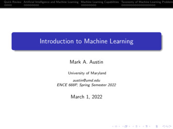
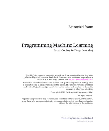
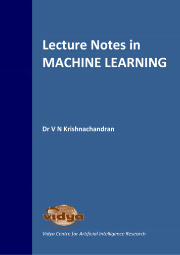
2. What is Machine Learning?“Optimizing a performance criterion using example data and past experience”,said by E. Alpaydin [8], gives an easy but faithful description about machine learning.In machine learning, data plays an indispensable role, and the learning algorithm isused to discover and learn knowledge or properties from the data. The quality orquantity of the dataset will affect the learning and prediction performance. Thetextbook (have not been published yet) written by Professor Hsuan-Tien Lin, themachine learning course instructor in National Taiwan University (NTU), is also titledas “Learning from Data”, which emphasizes the importance of data in machinelearning. Fig. 1 shows an example of two-class dataset.2.1 Notation of DatasetBefore going deeply into machine learning, we first describe the notation ofdataset, which will be used through the whole section as well as the tutorial. There aretwo general dataset types. One is labeled and the other one is unlabeled: Labeled dataset Unlabeled dataset:X { x ( n ) Rd }nN 1 , Y { y ( n ) R}nN 1: X { x ( n ) Rd }nN 1, where X denotes the feature set containing N samples. Each sample is ad-dimensional vector x ( n ) [ x1( n ) , x2( n) ,., xd( n) ]T and called a feature vector or featuresample, while each dimension of a vector is called an attribute, feature, variable, orelement. Y stands for the label set, recording what label a feature vector correspondsto (the color assigned on each point in Fig. 1). In some applications, the label set isunobserved or ignored. Another form of labeled dataset is described as{ x ( n ) Rd , y ( n ) R}nN 1 , where each { x ( n ) , y ( n ) } is called a data pair.2.2 Training Set and Test SetIn machine learning, an unknown universal dataset is assumed to exist, whichcontains all the possible data pairs as well as their probability distribution of4
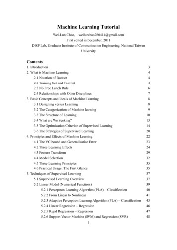
appearance in the real world. While in real applications, what we observed is only asubset of the universal dataset due to the lack of memory or some other unavoidablereasons. This acquired dataset is called the training set (training data) and used tolearn the properties and knowledge of the universal dataset. In general, vectors in thetraining set are assumed independently and identically sampled (i.i.d) from theuniversal dataset.Fig. 1An example of two-class dataset is showed, where two measurements ofeach sample are extracted. In this case, each sample is a 2-D vector [9].In machine learning, what we desire is that these learned properties can not onlyexplain the training set, but also be used to predict unseen samples or future events. Inorder to examine the performance of learning, another dataset may be reserved fortesting, called the test set or test data. For example, before final exams, the teachermay give students several questions for practice (training set), and the way he judgesthe performances of students is to examine them with another problem set (test set). Inorder to distinguish the training set and the test set when they appear together, we usetrainandtestto denote them, respectively.We have not clearly discussed what kinds of properties can be learned from thedataset and how to estimate the learning performance, while the readers can just leaveit as a black box and go forth. In Fig. 2, an explanation of the three datasets above ispresented, and the first property a machine can learn in a labeled data set is shown, theseparating boundary.5
Fig. 2An explanation of three labeled datasets. The universal set is assumed toexist but unknown, and through the data acquisition process, only a subset ofuniversal set is observed and used for training (training set). Two learned separatinglines (the first example of properties a machine can learn in this tutorial) are shown inboth the training set and test set. As you can see, these two lines definitely give 100%accuracy on the training set, while they may perform differently in the test set (thecurved line shows higher error rate).2.3 No Free Lunch RuleIf the learned properties (which will be discussed later) can only explain thetraining set but not the test or universal set, then machine learning is infeasible.Fortunately, thanks to the Hoeffding inequality [10] presented below, the connectionbetween the learned knowledge from the training set and its availability in the test setis described in a probabilistic way:2P[ ] 2e 2 N .(1)In this inequality, N denotes the size of training set, and and describe how theleaned properties perform in the training set and the test set. For example, if thelearned property is a separating boundary, these two quantities usually correspond tothe classification errors. Finally, is the tolerance gap between and . Details ofthe Hoeffding inequality are beyond the scope of this tutorial, and later an extendedversion of the inequality will be discussed.6
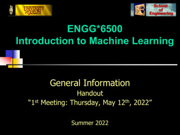
(a)(b)(c)Fig. 3The no free lunch rule for dataset: (a) is the training set we have, and (b), (c)are two test sets. As you can see, (c) has different sample distributions from (a) and(b), so we cannot expect that the properties learned from (a) to be useful in (c).While (1) gives us the confidence on applying machine learning, there are somenecessary rules to ensure its availability. These rules are called the “no free lunchrules” and are defined on both the dataset and the properties to learn. On the dataset,the no free lunch rules require the training set and the test set to come from the samedistribution (same universal set). And on the properties, the no free lunch rules ask theusers to make assumptions on what property to learn and how to model the property.For example, if the separating boundary in a labeled dataset is desired, we also needto define the type of the boundary (ex. a straight line or a curve). On the other hand, ifwe want to estimate the probability distribution of an unlabeled dataset, thedistribution type should also be defined (ex. Gaussian distribution). Fig. 3 illustratesthe no free lunch rules for dataset.2.4 Relationships with Other DisciplinesMachine learning involves the techniques and basis from both statistics andcomputer science: Statistics: Learning and inference the statistical properties from given data Computer science: Efficient algorithms for optimization, model representation,and performance evaluation.In addition to the importance of data set, machine learning is generally composed ofthe two critical factors, modeling and optimization. Modeling means how to modelthe separating boundary or probability distribution of the given training set, and thenthe optimization techniques are used to seek the best parameters of the chosen model.7
Machine learning is also related to other disciplines such as artificial neuralnetworks, pattern recognition, information retrieval, artificial intelligence, data mining,and function approximation, etc. Compared to those areas, machine learning focusmore on why machine can learn and how to model, optimize, and regularize in orderto make the best use of the accessible training data.3. Basic Concepts and Ideals of Machine LearningIn this section, more details of machine learning will be presented, including thecategorization of machine learning and what we can learn, the goals we are seeking,the structure of learning process, and the optimization criterion, etc. To begin with, asmall warming up is given for readers to get clearer why we need to learn.3.1 Designing versus LearningIn daily life, people are easily facing some decisions to make. For example, if thesky is cloudy, we may decide to bring an umbrella or not. For a machine to makethese kinds of choices, the intuitive way is to model the problem into a mathematicalexpression. The mathematical expression could directly be designed from the problembackground. For instance, the vending machine could use the standards and securitydecorations of currency to detect false money. While in some other problems that wecan only acquire several measurements and the corresponding labels, but do not knowthe specific relationship among them, learning will be a better way to find theunderlying connection.Another great illustration to distinguish designing from learning is the imagecompression technique. JPEG, the most widely used image compression standard,exploits the block-based DCT to extract the spatial frequencies and then unequallyquantizes each frequency component to achieve data compression. The success ofusing DCT comes from not only the image properties, but also the human visualperception. While without counting the side information, the KL transform(Karhunen-Loeve transform), which learns the best projection basis for a given image,has been proved to best reduce the redundancy [11]. In many literatures, theknowledge acquired from human understandings or the intrinsic factors of problemsare called the domain knowledge. And the knowledge learned from a given trainingset is called the data-driven knowledge.8
3.2 The Categorization of Machine LearningThere are generally three types of machine learning based on the ongoingproblem and the given data set, (1) supervised learning, (2) unsupervised learning,and (3) reinforcement learning: Supervised learning: The training set given for supervised learning is thelabeled dataset defined in Section 2.1. Supervised learning tries to find therelationships between the feature set and the label set, which is theknowledge and properties we can learn from labeled dataset. If each featurevector x is corresponding to a label y L, L {l1 , l2 ,., lc } (c is usually rangedfrom 2 to a hundred), the learning problem is denoted as classification. On theother hand, if each feature vector x is corresponding to a real value y R , thelearning problem is defined as regression problem. The knowledge extractedfrom supervised learning is often utilized for prediction and recognition. Unsupervised learning: The training set given for unsupervised leaning is theunlabeled dataset also defined in Section 2.1. Unsupervised learning aims atclustering [12], probability density estimation, finding association amongfeatures, and dimensionality reduction [13]. In general, an unsupervisedalgorithm may simultaneously learn more than one properties listed above, andthe results from unsupervised learning could be further used for supervisedlearning. Reinforcement learning: Reinforcement learning is used to solve problems ofdecision making (usually a sequence of decisions), such as robot perception andmovement, automatic chess player, and automatic vehicle driving. This learningcategory won’t be discussed further in this thesis, and readers could refer to [14]for more understanding.In addition to these three types, a forth type of machine learning category,semi-supervised learning, has attracted increasing attention recently. It is definedbetween supervised and unsupervised learning, contains both labeled and unlabeleddata, and jointly learns knowledge from them. Figs. 4-6 provide clear comparisonsamong these three types of learning based on nearly the same training set, and thedotted lines show the learned knowledge.9
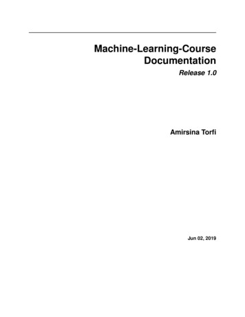
3.3 The Structure of LearningIn this subsection, the structure of machine learning is presented. In order toavoid confusion about the variety of unsupervised learning structures, only thesupervised learning structure is shown. While in later sections, several unsupervisedlearning techniques will still be mentioned and introduced, and important referencesfor further reading are listed. An overall illustration of the supervised learningstructure is given in Fig. 7. Above the horizontal dotted line, an unknown targetfunction f (or target distribution) that maps each feature sample in the universaldataset to its corresponding label is assumed to exist. And below the dotted line, atraining set coming from the unknown target function is used to learn or approximatethe target function. Because there is no idea about the target function or distribution f(looks like a linear boundary or a circular boundary?), a hypothesis set H is necessaryto be defined, which contains several hypotheses h (a mapping function ordistribution).(a)(b)Fig. 4Supervised learning: (a) presents a three-class labeled dataset, where thecolor shows the corresponding label of each sample. After supervised learning, theclass-separating boundary could be found as the dotted lines in (b).Insides the hypothesis set H, the goal of supervised learning is to find the best h,called the final hypothesis g, in some sense approximating the target function f. Inorder to do so, we need further define the learning algorithm A, which includes theobjective function (the function to be optimized for searching g) and theoptimization methods. The hypothesis set and the objective function jointly modelthe property to learn of the no free lunch rules, as mentioned in Section 2.3. Finally,the final hypothesis g is expected to approximate f in some way and used forfuture prediction. Fig. 8 provides an explanation on how hypothesis set works withthe learning algorithm.10
(a)(b)Fig. 5Unsupervise learning (clustering): (a) shows the same feature set as abovewhile missing the label set. After performing the clustering lagorithm, threeunderlined groups are discovered from the data in (b). Also, users can perform otherkonds of unsupervides learning algorithm to learn different kinds of knowledge (ex.Probability distributuion) from the unlabeled dataset.(a)(b)Fig. 6Semi-supervised learning. (a) presents a labeled dataset (with red, green,and blue) together with a unlabeled dataset (marked with black). The distribution ofthe unlabeled dataset could guide the position of separating boundary. After learning,a different boundary is depicted against the one in Fig. 4.There are three general requirements for the learning algorithm. First, thealgorithm should find a stable final hypothesis g for the specific d and N of thetraining set (ex. convergence). Second, it has to search out the correct and optimal gdefined through the objective function. The last but not the least, the algorithm isexpected to be efficient.11
Fig. 7The overall illustration of supervised learning structure: The part above thedotted line is assumed but inaccessible, and the part below the line is trying toapproximate the unknown target function (f is the true target function and g is thelearned function).Fig. 8An illustration on hypothesis set and learning algorithm. Take linearclassifiers as an example, there are five hypothesis classifiers shown in the up-leftrectangle, and in the up-right one, a two-class training set in shown. Through thelearning algorithm, the green line is chosen as the most suitable classifier.12
3.4 What are We Seeking?From the previous subsection, under a fixed hypothesis set H and a learningalgorithm A, learning from labeled dataset is trying to find g that best approximatesthe unknown f “in some sense”. And in this subsection, the phrase in the quotes isexplained for both supervised and unsupervised learning: Supervised learning: In supervised learning, especially for the classificationcase, the desired goal (also used as the performance evaluation) of learning is tofind g that has the lowest error rate for classifying data generated from f. Thedefinition of classification error rate measured on a hypothesis h is shown asbelow:E ( h) , where 1 N true 1(n)(n)y h(x), N n 1 false 0(2)stands for the indicator function. When the error rate (2) is defined onthe training set, it is named the “in-sample error Ein (h) ”, while the error ratecalculated on the universal set or more practically the (unknown or reserved)test set is named the “out-of-sample error Eout (h) ”. Based on these definitions,the desired final hypothesis g is the one that achieves the lowest out-of-sampleerror over the whole hypothesis set:g arg min Eout (h).h(3)While in the learning phase, we can only observe the training set, measure Ein (h) ,and search g based on the objective function. From the contradiction above, aquestion the readers may ask, “What is the connection among the objectivefunction, Ein ( g ) , and Eout ( g ) , and what should we optimize in the learningphase?”As mentioned in (1), the connection between the learned knowledge fromthe training set and its availability on the test set can be formulated as aprobability equation. That equation is indeed available when the hypothesis setcontains only one hypothesis. For more practical hypothesis sets which maycontain infinite many hypotheses, an extended version of (1) is introduced as:Eout ( g ) Ein ( g ) O(dVClog N ), with probability 1 .N13(4)
This inequality is called the VC bound (Vapnik–Chervonenkis bound), wheredVC is the VC dimension used as a measure of model (hypothesis set andobjective function) complexity, and N is the training set size. The VC boundlisted here is a simplified version, but provides a valuable relationship betweenEout ( g ) and Ein ( g ) : A hypothesis g that can minimize Ein (h) may induce a lowEout ( g ) . The complete definition of the VC dimension is beyond the scope ofthis tutorial.Based on the VC bound, a supervised learning strategy called empiricalrisk minimization (ERM) is proposed to achieve low Eout ( g ) by minimizingEin ( g ) :g arg min Ein (h).h(5)ERM is probably the most widely-used strategy is supervised learning, andEin (h) is the first objective function presented in this tutorial. In fact, anobjective function can be separated into a loss function and a penalty function.The loss function measures the classification error defined on the training set,while the penalty function gives each hypothesis a priority. Before Section 4.4,the penalty term is set as a constant and can be ignored. There are other kinds ofsupervised learning strategies seeking the minimum Eout ( g ) based on theoremsapart from the VC bound and will be mentioned in Section 3.6.For regression problem, the widely-used strategy is to minimize the rootmean square (RMS) between the predicted label and the ground truth label (thelabel provided by the dataset):E ( h) 21 N (n)y h( x ( n ) ) . N n 1(6)Unsupervised learning: Apart from supervised learning, the strategies ofunsupervised learning are very diverse. Some unsupervised learning algorithmsexploit probabilistic distribution model and find the best distribution parametersthrough maximum likelihood estimation (MLE), maximum a posterior (MAP),or a more complicated Bayes methods. On the other hand, algorithms withoutprobability models may learn knowledge based on statistical measurement,quantization error, variance preserving, or entropy gap, etc.3.5 The Optimization Criterion for Supervised LearningAs mentioned in Section 2.4, modeling and optimization are the two mainfactors of machine learning. The modeling contains the choice of hypothesis set H and14
the objective function, and optimization is performed to find the final hypothesis g inH, which reaches the minimum or maximum of the objective function (if necessary,within the user-defined number of iteration). Given a training set, there are indeedmany kinds of models to choose. In order to avoid confusion, in this section weassume the hypothesis set is fixed, and what we want to do is searching g based on theselected objective function. In Section 4, we will introduce the methods to choose amodel for the training set and problem at hand, and in Section 5, the types ofhypothesis sets and their corresponding objective functions are discussed in moredetailed.We first focus on the hypothesis set of linear classifiers and show how theoptimization methods interact with the choices of objective functions. The generalform of the linear classifier for two-class classification problems ( y ( n ) [ 1,1] ) isformulated as below:h( x ( n ) ) sign(wT x(n) c) ,(7)where c is some constant, w is a (d 1)-dimensional vector w [w0 , w1 ,., wd ]T , andx [1, x1 , x2 ,., xd ]T is the extended version of x also with (d 1) dimensions. Thevector w stands for the classifier parameters, and the additional 1 in x is used tocompute the offset of the classification line. Based on the goal of ERM introduced inSection 3.4, the objective function is the in-sample error term (or say the loss term,calculating how many training samples are wrongly predicted) and the optimizationmethod is used to find a linear classifier to minimize the objective function. Fig. 9shows a linearly-separable training set as well as the corresponding final hypothesisg. As you can see, there are many hypotheses that could achieve zero error.Fig. 9An example of two-class classification problem using linear classfiers,where the training set is linearly-separable.15
Fig. 10 The objective (in-sample error rate) considering only a sample withy ( n ) 1 based on linear classfiers. The x-axis denotes the inner product of theextended feature vector and the parameter vector of the linear classifier. As shown, theobjective function is non-continuous around wT x(n) 0.If we simplify (2) and just look at one sample without normalization, the errorterm will become:loss ( n ) ( g ) y ( n ) g ( x ( n ) ) .(8)Fig. 10 shows this one-sample objective function for a sample with y ( n ) 1 . As can beseen, the fuction is non-continuous around wT x(n) 0 and flat in the other ranges, sothe use of differentiation-based (iterative) optimization methods is nearly out of work.For example, if the attained w brings wT x(n) 0 for y ( n ) 1 at the current iteration,with zero gradients according to w, the optimization algorithm has no idea to adjustthe current w towards lower error rate. Fig. 11 illustrates this problem for alinear-separable training set.Differentiation-based optimization methods are probably the most widely-usedoptimization techniques in machine learning, especially for objective functions thatcan be directly written as a function form of the traning samples and the classifier orregressor parameters w (not always in the vector form). The popular gradient descent,stochastic gradeint descent, Newton’s method, coordinate descent, and convexoptimization are of this optimization category. The differentiation-based methods areusually performed in the iterative manner, which may suffer from the local optimalproblem. Besides, some of them cannot even reach the exact local optimal due toconvergence concern, where slow updating and small vibration usually occur aroundthe exact optimal parameters. Despite these drawbacks, the optimization category is16
popular because of its intuitive geometrical meaning and usually easy to start with bysimple caluculus such as the Taylor’s expansion.Fig. 11Assume at the current iteration, the attained w and one of the desired w areshown as the black and the gray dotted lines, the optimization algorithm may haveno idea on how to adjust w towards its desired quantities.The basic concerns to exploit this optimization category are the “differentiability”of the objective function and the “continuity” of the parameter space. The objectivefunction may have some non-continuous or undifferentiable points, while it should atleast be in a piecewise differentiable form. In addition to differentiability, we alsoexpect that the fuction has non-zero gradients along the path of optimization, and thezero gradients only happen at the desired optimal position. As shown in 錯誤! 找不到參照來源。, the in-sample error rate of linear classifiers is neither continuous norwith non-zero gradients along the optimization path. This non-continuous objectivefunction may still be solved by some other optimization techniques such as theperceptron learning algorithm, the neural evolution, and the genetic algorithm, etc.,while they are either much more complicated, require more computational time, or areonly available in certain convergence-guarantee conditions. The objective functionshould not be confused with the classifier or regressor functions. The second term isthe function for predicting the label of the feature vector, and the first term is thefunction used to find the optimal parameters of classifiers or regressors.To make differentiation-based optimization methods available for ERM in thelinear classifier case, we need to modify the in-sample error term into some otherapproximation functions that is (piecewise) differentiable and continuous. There aremany choices of approximation functions (denoted as Eapp (h) ), and the onlyconstraint on them is made as below:17
Eapp (h) Ein (h)(9), which means the in-sample error is always upper-bounded by the approximationfunction. Based on this modification, the learning goal and procedure for ERM isreformulated. The original learning goal aims at finding g which approaches thetarget function f through minimizing Eout (h) . Because of the inaccessibility to the testand universal set, the learning phase turns to optimize Ein (h) with g by ERM, andexpects g to approach g ( Eout ( g ) Eout ( g * ) ) through the VC bound introduced in (4).Furthermore, due to the difficulty of optimizing Ein (h) , an approximation functionEapp (h) is defined to take place of Ein (h) . Trough searching g which optimizes Eapp (h)with the constraints defined in (9), we expect the final hypothesis g could achieve lowEin ( g )
dataset, which will be used through the whole section as well as the tutorial. There are two general dataset types. One is labeled and the other one is unlabeled: Labeled dataset : () {} 1 n d N XR x n, () 1 nN Y y R n Unlabeled dataset : {} 1 n d N XR x n, where X denotes the feature set containing N samples. Each sample is a d-dimensional vector