Transcription
First version: June 18, 2004Revised: January 24, 2008PATRICIA LEDESMA LIÉBANASAS programming skillsThis document is not a self-paced SAS tutorial; rather, it focuses on data management skillsand features of SAS that are helpful in a research context. However, it does provide the basicelements of the SAS Language. If you have some previous programming experience, the skillslisted here should be easy to understand. For a comprehensive SAS tutorial, please refer to “TheLittle SAS Book” by Delwiche and Slaughter, available in the Research Computing library (room4219).Contents1. SYNTAX RULES2. BASIC PARTS OF A SAS PROGRAM3. TYPES OF DATA FILES4. PROVIDING DATA IN THE PROGRAM5. CREATING VARIABLES6. SAS OPERATORS AND FUNCTIONS7. READING “RAW” DATA – EXTERNAL FILES8. COMBINING DATASETS8.1. Appending datasets8.2. Merging datasets8.3. PROC SQL9. USING PROCEDURES TO GENERATE DATASETS10. LIBNAMES AND SAS DATASETS11. BY PROCESSING12. CREATING COUNTERS13. LAGS IN PANEL DATASETS14. ARRAYS15. WRITING ASCII OUTPUT DATASETS15.1. Plain ASCII files: FILE and PUT statements15.2. Creating or reading CSV files: EXPORT and IMPORT16. USEFUL PROCEDURES16.1. “Flipping” your data: PROC TRANSPOSE16.2. Dealing with rolling windows: PROC EXPAND17. ODS TO GENERATE CUSTOMIZED DATASETS FROM PROCS18. IML – INTERACTIVE MATRIX LANGUAGE19. MACROS – AN EXAMPLE20. USING SAS MANUALS 2004-2008 Patricia Ledesma Liébana22334566677991011111212121313131314151618
SAS PROGRAMMING SKILLS1. Syntax rules All commands end in a semi-colon SAS statements are not case sensitive. You may use upper or lower case. Variables names can be upper or lower case. When you refer to "external" file name, it is case-sensitive (interaction with UNIXoperating system) Commands can extend over several lines as long as words are not split You may have more than one command per line SAS name rules (for datasets and variables): up to 32 characters long; must start witha letter or an underscore (“ ”). Avoid special characters.2. Basic parts of a SAS program2 There are two basic building blocks in a SAS program: DATA ‘steps’ and PROC(procedures). SAS procedures do not require the execution of a data step before them. In addition, OPTIONS to control appearance of output and log files. The DATA step is where you manipulate the data (creating variables, recoding,subsetting, etc). The data step puts the data in a format SAS can understand. A SAS data file can have up to three parts: (a) the headers – descriptive informationof the dataset’s contents; (b) the matrix of data values; and (c) if created, indexes.Indexes are saved to separate “physical” files, but SAS considers it part of the datafile. Thus, if an index exists, it should not be removed from the directory where thedata file resides. Version 8 data files have the extension “.sas7bdat”, while index fileshave extension “.sas7bndx”. Most data files in WRDS have indexes. SAS reads and executes a data step statement by statement, observation byobservation. All the variables in the portion of memory that processes the currenteach observation (input buffer or program data vector, depending on whether you arereading “raw” data or a SAS data file) are reset to missing in each iteration of thedata step. The RETAIN statement prevents this from happening. Missing values: Generally, missing values are denoted by a period (“.”). Mostoperators propagate missing values. For example, if you have three variables (v1, v2,v3) and for observation 10, v2 is missing, creating total v1 v2 v3 will result in amissing value for observation 10 [if you would like the sum of the non-missingvalues, use the SUM function: total sum(v1,v2,v3)]. However, for comparisonoperators ( , , or ), SAS treats missing values as infinitely negative numbers(- ) [unlike Stata, which treats them as infinitely positive]KELLOGG SCHOOL OF MANAGEMENT
SAS PROGRAMMING SKILLS PROCs are used to run statistics on existing datasets and, in turn, can generatedatasets as output. Output data sets are extremely useful and can simplify a great dealof the data manipulation. DATA step and PROC boundary: Under Windows, all procedures must end with a“RUN;” statement. In UNIX, this is not necessary since SAS reads the entire programbefore execution. Does, it determines DATA step boundaries when it encounters aPROC and knows the boundary of a PROC when it is followed by another PROC ora DATA step. The one exception to this rule is in the context of SAS macros, whereyou may need to add the “RUN;” statement.3. Types of data files SAS distinguishes two types of files: “internal” (created by SAS) and “external”.Referring to files in SAS maybe the most complicated point in learning SAS. Here,the conventions date to mainframe systems. In brief, files external to SAS are ASCII(or text) files and files generated by other applications (such as Excel, SPSS, etc).Files internal to SAS are divided into “temporary” or “scratch” files, which exist onlyfor the duration of the SAS session, and “permanent” files, which are saved to disk. ASCII External Files generated by other programsFiles in SAS Internal Temporary, " scratch" - one level names Permanent - two level names (libref.name) SAS scratch files are created and held until the end of the session in a specialdirectory created by SAS in a scratch area of the workstation. When SAS finishesnormally, all the files in this directory are deleted. SAS permanent files are written to a “SAS library”, which is simply a directory in thesystem with a collection of SAS data files. In the program, the directory is assigned anickname, called a “libref” in the manuals, with a LIBNAME statement.Subsequently, to refer to a permanent file, you type the libref, followed by a period,followed by a name. The examples below build a data file. Until a complete version of the file is created,all intermediate data files are “scratch” files. We ignore the LIBNAME statementuntil the sample code in section 7.4. Providing data in the programUse a text editor to create the following program (call the file “ipos.sas”):data ipo;input ticker offer prc offer amount open prcKELLOGG SCHOOL OF MANAGEMENT3
SAS PROGRAMMING SKILLSdate public mmddyy8.;format date public yymmddn8.;cards;ACAD 7 37.5 7.44 05/27/04CYTK 13 86.3 14.5 04/29/04CRTX 7 48 7.26 05/27/04EYET 21 136.5 30 01/30/04;proc sort data ipo; by descending offer amount;proc print data ipo;title 'Recent IPOs';Note that the name of the date variable is followed by “mmddyyn8.”. This is a date“informat”, an instruction that tells SAS how to read the values. SAS will read the dates into SASdates (number of days elapsed since January 1, 1960), enabling you to do calculations with thedate. The format statement includes a SAS format, an instruction to SAS on how to display thedate (internally, it keep the number of days since 01/01/1960). The “n” in the format standsindicates that we do not want any separators between the year, month and day (for a slash, theformat would be yymmdds10.).To run the program, exit the text editor, type the following command at the UNIX promptand hit enter to execute:sas iposSAS will create two files: ipos.log: The LOG file has all the messages, errors and warnings that the SAScompiler has issued during execution of your program. Always check it. ipos.lst: The listing file contains any “printed” output generated by a procedure.Use the UNIX “more” command to browse these files.5. Creating variablesNew variables can be defined in the data step. For example, in the previous program, type thefollowing statement after the INPUT statement (between INPUT and CARDS):open offer ret open prc/offer prc;Run the program again to view the results. SAS has a wide range of functions that can also beused to modify your data.4KELLOGG SCHOOL OF MANAGEMENT
SAS PROGRAMMING SKILLS6. SAS operators and functionsFor a complete listing of functions and their syntax, refer to the SAS/BASE “SAS LanguageReference: Dictionary” manual. For detailed explanations of the precedence each operator takesand how SAS expressions are built, refer to the SAS/BASE “SAS Language Reference:Concepts” manual. The list below only includes some of the functions I use most.ArithmeticLogicalAs in Excel: , -, *, /And: & or ANDEqual: Exponentiation: **Or: or ORLess than: or LTNot: or NOTComparisonLess than or equal: or LEGreater than: or GTGreater than or equal: or GENot equal to: or NEAn additional important operator not included in the categories above, is the concatenationoperator, which creates one alphanumeric by concatenating two character strings: Functions work across variables (in rows). Some important functions: ABS(x): absolute value DIFn(X): difference between argument and its n-th lag EXP(x): raises e to x power. FLOOR(x): integer that is less than or equal to x. Same results as INT(x) INDEX(argument, excerpt) searches an argument and returns the position of the firstoccurrence. LAGn(x): lagged values from queue (LAG(.) is first lag)). LOG(x): natural log of x (LOG2(x) logarithm to the base 2, LOG10(x) logarithm tothe base 10) MAX(x), MIN(x): Maximum and minimum MEAN(X), SUM(X) N(x) number of non missing values NMISS(x) number of missing values SUBSTR(argument, position, length) retrieves a portion of a given stringKELLOGG SCHOOL OF MANAGEMENT5
SAS PROGRAMMING SKILLS7. Reading “raw” data – external filesTo read data from an ASCII file, you must specify the location of the file using either theFILENAME statement or the INFILE statement.We will use the following sample data file: ple531/sastraining/sampledata.prnIn the next example, we will use the INFILE version, where the location of the external file isreferenced in quotes:data t1;infile ' ple531/sastraining/sampledata.prn' firstobs 2;input yearticker data6data12fiction;proc print data t1;Note: The FILENAME would assign a “fileref” or handle to the external file, which wouldthen be used by the INFILE statement. The first lines of the code would be written as follows:filename raw ' ple531/sastraining/sampledata.prn';data t1;infile raw firstobs 2;etc.Note that “raw” is an arbitrary nickname for the external file, which is then used in theINFILE statement instead of the file location. The FILENAME command is structured like theLIBNAME command in section 7 and, if your program is reading several external files, it mightbe a more organized way of writing the program: declare all the external file names at thebeginning of the program (a sequence of FILENAME statements), making easier replication ofresults if you must move the data files and programs to a different computer.8. Combining datasetsThere are two common types of dataset operations: appending datasets with the samevariables or combining (merging) datasets with different variables.8.1. Appending datasetsIn “ ple531/sastraining/additionaldata.txt” there are three additional years of sample data,with four of the same variables as “sampledata.prn”. To append or concatenate these datasets,first add the following statements to read the additional data into a SAS dataset:6KELLOGG SCHOOL OF MANAGEMENT
SAS PROGRAMMING SKILLSdata t2;infile ' ple531/sastraining/additionaldata.txt' firstobs 2;input year ticker data6 data12;Next, concatenate both files with a new data step:data t3;set t1 t2;Note: This can also be done with APPEND procedure, which is more resource efficient.Instead of the additional data step, you can try:proc append base t1 data t2;In general, proc append will be faster than the data step: the data step will read bothdatasets (t1 and t2), while proc append will only read the second (t2, the dataset beingappended to the end of t1, the base dataset).8.2. Merging datasetsFile “ ple531/sastraining/moredata.txt” has an additional variable, a fictional dummy for fairtrade coffee. It also includes the tickers. To merge these data with the rest of our coffee data:data t4;infile ' ple531/sastraining/moredata.txt';input ticker fair;proc sort data t4; by ticker;proc sort data t3; by ticker year;data t5;merge t3 t4;by ticker;One thing to keep in mind to control the result of the merge, is that SAS keeps track of thedataset that contributes to each observation with some internal dummies. Using the “IN ” datasetoption (for example, “merge t3 (in a) t4 (in b);”) it is possible to control whatobservations are in the final dataset. By default, it would be all observations (from t3 and t4).Using an IF statement such as the one below writes only those observations for which bothdatasets contributed. Similarly, one could specify “in a;”, “in b;”, “if not b;”, etc.data t5;merge t3 (in a) t4 (in b);by ticker;if a and b;8.3. PROC SQLPROC SQL is the SAS implementation of the Standard Query Language (SQL) standard towork with databases and is used in Oracle, Microsoft SQL Server, Microsoft Access and otherdatabase systems. PROC SQL is a powerful language that allows sophisticated merges. WhenKELLOGG SCHOOL OF MANAGEMENT7
SAS PROGRAMMING SKILLSyou merge datasets with PROC SQL you do not need to sort them. Given that most files inWRDS are indexed, PROC SQL also works fast when creating queries on CRSP and Compustat,for example. Consider the example below, from the WRDS sample file “ina.sas” to retrieve datafrom the Compustat Industrial file.To end PROC SQL you must type use the QUIT statement. The SQL query is between PROCSQL and QUIT (as a very long statement). Unlike the rest of SAS, datasets are called “tables”,while variable names now have two levels (e.g., inanames.coname): the first level denotes thetable of origin (dataset “inanames”), while the second level is the variable name itself(“coname”). There is no reference to SAS libnames except in the “FROM” part of the SQL query.In the example below, the query itself has been broken into lines for convenience. The firstline defines the dataset that will be created (temp2) by selecting variables from dataset inanames(coname and iname) and dataset “temp” (all variables). The second line of the query defines thesources of the datasets: temp is a temporay dataset (defined in earlier SAS statements) and inamesis in the “comp” library (the libref assigned to the location of Compustat files in WRDS). Finally,the WHERE portion of the query defines how the merge is done. In this example, observationsfrom temp are matched to observations of inanames on the basis of CNUM (CUSIP issuernumber) and CIC (the issue number and check digit). Note that the variables in temp are namedleft of the equal sign; this implicitly defines a “left join” in which all the records of temp will bepreserved (whether there is matching Compustat data or not) and only matching records of theCompustat inanames file.PROC SQL;CREATE TABLE temp2 AS SELECTinanames.coname, inanames.iname, temp.*FROM temp, comp.inanamesWHERE temp.cnum inanames.cnum AND temp.cic inanames.cic;QUIT;To achieve the same with a MERGE statement, assuming both datasets are sorted by CNUMand CIC, the DATA step would read:data temp2;merge temp (in a) comp.inanames;if a;Given that “inanames” is a large file and that the DATA step will copy each mergedobservation before evaluating the IF statement, this option is less efficient than the PROC SQLversion.The next example shows a more complex SQL statement in which observations from TAQconsolidated trades (test) and consolidated quotes (test2) are matched based on the date andsymbol, as well as time stamp for each record. In this case, for each trade, we match all the quotesin a 10 second window. Note that variable “secs” is a calculation based on variables fromdifferent datasets. Also, notice that the time stamp variable was renamed on the fly.proc sql;create table combined asselect test.symbol, test.date, test.price, test.size,test2.bid, test2.ofr, test2.bidsiz, test2.ofrsiz,8KELLOGG SCHOOL OF MANAGEMENT
SAS PROGRAMMING SKILLStest.ct time, test2.cq time,(test2.cq time-test.ct time) as secsfrom test(rename (time ct time)) left jointest2(rename (time cq time))on -10 (ct time-cq time) 10where test.symbol test2.symbol and test.date test2.date;quit;Some limitations of PROC SQL are: (i) it can merge up to 16 tables, versus SAS normal limitof 100; (ii) if you are merging many tables, PROC SQL can be slower relative to using a MERGEstatement.9. Using procedures to generate datasetsMost (if not all) SAS procedures can generate output datasets that you can use for furtherprocessing (merge with another datasets, etc), with either an OUT option or an OUTEST option. Note that you can use DATA step options when you create these datasets.proc sort data t5; by fair;proc means data t5 noprint;var data6 data12;by fair;output out t6 (drop freq type ) mean / autoname;proc print data t6;The resulting dataset can be merged with the original data to “propagate” the mean values,allowing us to use it for further computations:proc sort data t5; by fair;data spiff.t7;merge t5 t6;by fair;For more options to generate output datasets from SAS procedures, see section 16 below, onthe “Output Delivery System” (ODS).10. LIBNAMES and SAS datasetsSAS creates two types of SAS “system” data files: temporary (“scratch” or “work” files) o“permanent”. Both types of files are SAS data files. Physical SAS files have the “sas7bdat”extension for SAS versions 7 and up.Temporary files are files created during a SAS session (either in interactive mode or duringthe execution of a SAS program. Temporary files are named in the program with a one-levelname. For example in “DATA oranges”, the dataset “oranges” is temporary. If the program endssuccessfully, the “oranges” file will be deleted by SAS at the end. If the execution fails,temporary files will not be deleted.KELLOGG SCHOOL OF MANAGEMENT9
SAS PROGRAMMING SKILLSIn each SAS installation, there is a default location for the work directory, where temporaryfiles are created during a session. In Kellogg’s UNIX server, temporary files are directed to“/scratch/sastemp”. This location can be changed by specifying the “-work” option beforeexecution:sas –work /someotherpath prognameAll default options for SAS are stored in a configuration file (sasv8.cfg) in the SAS programdirectory.“Permanent” files are SAS files named with a two-level name during the program. The firstlevel of this name is a handle or “libref” that associates the dataset with a specific directory whereit will be created and stored. The libref is created in a LIBNAME statement. The followingexample associates the “ /training” directory to the libref “spiff”. The libref is then used to writedataset “t7” to the directory named in the LIBNAME statement.libname spiff ' /training';data spiff.t7;merge t5 t6 (drop freq type );by fraud;11. BY processingThere are many operations that require handling the data in groups of observations, as definedby common values of one or more variables. Most procedures, if not all, allow BY and/or CLASSstatements. BY was also used above for merging data. The following example illustrates anotheruse of BY-processing in a data step.To use BY-processing in a data step, first you data must be sorted according to the variablesneeded in the BY statement. When the BY statement is invoked in the DATA step, SASautomatically creates a set of internal dummy variables that identify the boundaries of eachgroup. In the following example, it will create four dummy variables: first.sic, last.sic,first.permno, and last.permno. First.sic takes a value of one for the first observation in every SICcode, and is zero otherwise. Last.sic will be one in the last observation of every SIC code andzero otherwise.These internal variables can be used for a variety of purposes. In the example below, we arekeeping the last observation of every “permno”, and in the example that follows in section 12, weuse the internal variables to create a counter.PROC SORT DATA t1; BY sic permno date;DATA test;SET t1;BY sic permno;IF LAST.permno THEN OUTPUT;10KELLOGG SCHOOL OF MANAGEMENT
SAS PROGRAMMING SKILLS12. Creating countersThe following example creates a counter (called “qobs”) that counts that starts over for eachgroup. In this case, it is used to subset the first two observations in each group.PROC SORT DATA subset1;BY qdate DESCENDING idtdtd;DATA subset2;SET subset1;BY qdate DESCENDING idtdtd;RETAIN qobs;IF first.qdate THEN qobs 0;qobs qobs 1;if qobs in(1,2);The RETAIN statement is extremely powerful. SAS normally reads and processesobservation by observation in a data step. In each iteration, all the variables in the “program datavector” (the area of memory where the observation processed is being read) are reset to missingbefore reading the next observation. The RETAIN statement changes this behavior and keeps thevalue of the previous iteration. This is what enables the counter to increase from iteration toiteration.13. Lags in panel datasetsThe LAGn(argument) function can be used to create different lags of a variable. In thecontext of a panel dataset, the problem is the SAS DATA step does not distinguish betweendifferent cross-section units: if dealing with a monthly panel of securities, the lagged value ofvariable for the first observation of every cross-section unit (starting with the second one) will beset to the value of the variable for the last observation of the previous cross-section unit. A quicksolution is to use BY processing and “clean” the lags:PROC SORT DATA test; BY permno date;DATA test; set test;BY PERMNO;lagprc LAG(prc);IF FIRST.PERMNO then lagprc .;Higher order lags can be created by specifying the order in the function: LAG2(prc),LAG3(prc), etc.There is no “lead” function, but the LAG function can be used to create leads by using it aftersorting the dataset in descending order (BY permno DESCENDING date;)KELLOGG SCHOOL OF MANAGEMENT11
SAS PROGRAMMING SKILLS14. ArraysSAS arrays are named groups of variables within a DATA step that allow you to repeat thesame tasks for related variables. Arrays may have one or more dimensions. In the followingexample, we use only one dimension. Suppose you have received a data file where eachobservation is a firm (identified by permno) and 552 columns, each of them for a daily return,where missing values were coded as -99. Instead of writing 552 IF statements (“if ret1 -99then ret1 .; if ret2 -99 then ret2 .; etc”), you could define an array that groupsall 552 columns and the cycle through each variable replacing the values:data test;set retdata;array returns(552) ret1-ret552;do i 1 to 552;if returns(i) -99 then returns(i) .;end;drop i;There is more flexibility in SAS arrays than this example shows. For example, if the firmidentifier was a character variable (and all variables that you want in the array were numeric),instead of declaring the list of variables in the array as “array returns(552) ret1ret552”, you could declare it as “array returns(*) numeric ”. In this case, SAS willgroup all the numeric variables in the array and count how many there are (the array dimension).The DO statement would then be rewritten as “do i 1 to dim(returns);”15. Writing ASCII output datasets15.1. Plain ASCII files: FILE and PUT statementsWithin a data step, the combination of the FILE (naming the destination of the data) and PUT(which writes lines to the destination named in FILE) statements provides great flexibility. Youmay use it to generate anything from a plain ASCII data file to a LaTex table by including theproper formatting. The code below provides a very simple output file:data temp;set inststat;file 'spectruminst.dat';put cusip year totsh noinst;The PUT statement can be very refined. For example, if the data being written containsmissing values, then you may want to write a formatted PUT statement, in which each variablewill take a specific column location in the output file (e.g. cusip in columns 1-8 of the file, year incolumns 10-13, etc).12KELLOGG SCHOOL OF MANAGEMENT
SAS PROGRAMMING SKILLS15.2. Creating or reading CSV files: EXPORT and IMPORTPROC EXPORT and PROC IMPORT are procedures that allow SAS to create and readcomma-separated-values (CSV) files, which include headers. These files are easy to read inMatlab (csvread function – start reading in row 2 to avoid the header) and Stata (insheetcommand).proc export data tempoutfile "spectruminst.csv"dbms csvreplace;When you run a SAS program that includes a PROC EXPORT or a PROC IMPORT, be sureto specify the “-noterminal” option, as these procedures normally require X Windows:sas –noterminal program name16. Useful procedures16.1. “Flipping” your data: PROC TRANSPOSEPROC TRANSPORT, part of the SAS/BASE procedures, allows to restructure a datasetconverting variables into observations and vice versa.FILENAME spiff 'externaldata/multi.csv';PROC IMPORT DATAFILE spiff OUT test DBMS CSV;GETNAMES YES;*PROC CONTENTS DATA test; *PROC PRINT DATA test (OBS 10);PROC TRANSPOSE DATA test OUT test1 NAME ticker PREFIX date;VAR msft ibm ba xrx;ID date;PROC PRINT DATA test1;16.2. Dealing with rolling windows: PROC EXPANDThe following program uses PROC EXPAND (part of SAS/ETS) to compute a moving sumover a 3-month window. The example in question is for cumulative returns, calculated usingnatural logs. The data must be sorted by the group identifier (permno) and time identifier (date);the variable specified in the ID statement must be a SAS date or time. By default, PROCEXPAND uses the spline method to interpolate missing values; by specifying METHOD NONE,this is avoided. Finally, in the CONVERT statement, the options NOMISS and TRIMLEFT(which will set to missing the first two observations of every BY group) will ensure that all thecomputed cumulative returns include three dates. Otherwise, the first return for each permnowould be in the second date, computed with only two observations.DATA test; INFILE "rets2.txt";KELLOGG SCHOOL OF MANAGEMENT13
SAS PROGRAMMING SKILLSINPUT permno date YYMMN6. ret;FORMAT date YYMMN6.;logret LOG(ret 1);PROC PRINT DATA test (OBS 12);PROC EXPAND DATA test OUT out METHOD NONE;BY permno;ID date;CONVERT logret movsum / TRANSFORMOUT (NOMISS MOVSUM 3 TRIMLEFT 2);DATA out;SET out;cumret EXP(movsum)-1;PROC PRINT DATA OUT;This procedure can also compute statistics for centered windows, forward looking windows,lags, leads within a period, etc, so it can be a welcome alternative to a more complex data step.17. ODS to generate customized datasets from PROCsStarting with version 7, the “Output Delivery System” (ODS) allows the user to control eachportion of a procedure’s output. In particular (among many features), ODS allows the user tocreate datasets from specific portions of the output that could not be sent to a dataset with anOUT or OUTEST option. The complete ODS documentation is available in the SAS/BASEmanual “The Complete Guide to the SAS Output Delivery System”.To use ODS to create a dataset from a PROC statement:1. Find out how SAS calls the piece of output you need. For this, type “ODS TRACEON” before the PROC you need to examine, and “ODS TRACE OFF” after thePROC. Example:ods trace on;proc model data uspop;pop a / ( 1 exp( b - c * (year-1790) ) );fit pop start (a 1000 b 5.5 c .02);run;ods trace off;2. Run the program and examine the log file – it will include a listing of each object ofoutput sent to the LST file. For example, the table with parameter estimates in PROCMODEL is called “ParameterEstimates”.3. Use the object name to create the output file. Furthermore, you can “turn off” thelisting with the “ODS LISTING OFF” statement. This is extremely useful if you needto run the same procedure repeatedly for a large number of units – if you add theNOPRINT option to the procedure, no output will be written at all. Example:ods listing close;ods output ParameterEstimates d2 (drop Esttype);proc model data uspop;14KELLOGG SCHOOL OF MANAGEMENT
SAS PROGRAMMING SKILLSpop a / ( 1 exp( b - c * (year-1790) ) );fit pop start (a 1000 b 5.5 c .02);quit;ods listing; /* Allow output of PROC PRINT to be listed */proc print data d2;title "ODS output dataset";18. IML – Interactive Matrix LanguageSAS has a matrix language in which expressions are close to Matlab. You can read a SASdataset into a matrix or produce a dataset from a matrix – you may go back and forth betweenusing SAS data steps and procedures and using IML. Like in PROC SQL, you end the procedurewith a QUIT statement.The following example shows some functions in IML: (i) first, we read the “fake” datasetinto a matrix beta1; (ii) compute betax the inverse of beta1T*beta1 and print it (the matrix will beprinted in the LST file); (iii) define a column vector and a 2 by 2 matrix providing the data inIML; (iv) define a row vector with elements: x1, x2, x3; (v) create a new dataset, fake2, with thecontents of betax. The CREATE statement defines the dataset with the characteristics of the betaxmatrix, using newvars as the source of the column names. The APPEND statement “populates”the dataset with the data from the matrix. Note that the transpose symbol is the backquotecharacter, generally on the top left of a keyboard; alternatively, you may write t(beta1).data fake;input cusip v1 v2 v3;cards;a 1 34 65b 1 78 32c 2 12 01d 4 54 29;proc print data fake;proc iml;use fake;read all var num into beta1 [rowname cusip colname names];print beta1;betax inv(beta1 *beta1);print betax;columnvector {1,2,3,4};twobytwomatrix {1 2, 3 4};print columnvector, twobytwomatrix;newvars 'x1' : 'x3';create fake2 from betax [colname newvars];append from betax;close fake2;quit;proc print data fake2;KELLOGG SCHOOL OF MANAGEMENT15
SAS PROGRAMMING SKILLS19. Macros – an exampleThe next step in learning SAS is to learn macros. The SAS macro language allows you to runa program for different parameters, such as tickers, dates, etc. Build your macros step by step based on a program that works. At each stage of theprogram, use PROC PRINT to take a look at intermediate output. Add one macro variable at a time. Test extensively. For exampl
SAS distinguishes two types of files: "internal" (created by SAS) and "external". Referring to files in SAS maybe the most complicated point in learning SAS. Here, the conventions date to mainframe systems. In brief, files external to SAS are ASCII (or text) files and files generated by other applications (such as Excel, SPSS, etc).