Causal Discovery With Multi-Domain LiNGAM For Latent Factors PDF Free Download

1y ago

27 Views

1 Downloads

308.94 KB

7 Pages

Report/dmca

Download PDF

Transcription

Proceedings of the Thirtieth International Joint Conference on Artificial Intelligence (IJCAI-21)Causal Discovery with Multi-Domain LiNGAM for Latent FactorsYan Zeng1,2 , Shohei Shimizu2,3 , Ruichu Cai1 , Feng Xie4 ,Michio Yamamoto2,5 and Zhifeng Hao1,61Guangdong University of Technology2RIKEN3Shiga University4Peking University5Okayama University6Foshan Universityyanazeng013@gmail.com, shohei-shimizu@biwako.shiga-u.ac.jp, {cairuichu, xiefeng009}@gmail.com,m.yamamoto@okayama-u.ac.jp, zfhao@gdut.edu.cnAbstractof data alone, e.g., BuildPureClusters algorithm [Silva etal., 2006], or FindOneFactorClusters algorithm [Kummerfeld and Ramsey, 2016], to ascertain how many latent factors as well as the structure of latent factors. However,these algorithms can only output structures up to the Markovequivalence class for latent factors. Non-Gaussianity-basedmethods address this indistinguishable identification problemby taking the best of the non-Gaussianity of data. Specifically, Shimizu et al. [2009] leveraged non-Gaussianity andfirstly achieved identifying a unique causal structure betweenlatent factors based on the Linear, Non-Gaussian, AcyclicModels (LiNGAM) [Shimizu et al., 2006]. They transformedthe problem into the Noisy Independent Component Analysis(NICA). Recently, to avoid the local optima of the NICA, Caiet al. [2019] designed the so-called Triad constraints and Xieet al. [2020] developed the GIN condition. They both proposed a two-phase method to learn the structure or causal orderings among latent factors.Discovering causal structures among latent factorsfrom observed data is a particularly challengingproblem. Despite some efforts for this problem,existing methods focus on the single-domain dataonly. In this paper, we propose Multi-DomainLinear Non-Gaussian Acyclic Models for LAtentFactors (MD-LiNA), where the causal structureamong latent factors of interest is shared for all domains, and we provide its identification results. Themodel enriches the causal representation for multidomain data. We propose an integrated two-phasealgorithm to estimate the model. In particular, wefirst locate the latent factors and estimate the factorloading matrix. Then to uncover the causal structure among shared latent factors of interest, we derive a score function based on the characterizationof independence relations between external influences and the dependence relations between multidomain latent factors and latent factors of interest.We show that the proposed method provides locallyconsistent estimators. Experimental results on bothsynthetic and real-world data demonstrate the efficacy and robustness of our approach.1IntroductionLearning causal relationships from observed data, termed ascausal discovery, has been developed rapidly over the pastdecades [Pearl, 2009; Spirtes and Zhang, 2016; Peters et al.,2017]. In many scenarios, including sociology, psychology,and educational research, the underlying causal relations areusually embedded between latent variables (or factors) thatcannot be directly measured, e.g., anxiety, depression, or coping, etc [Silva et al., 2006; Bartholomew et al., 2008], inwhich scientists are often interested.Some approaches have been developed to identify thecausal structure among latent factors, which can be categorized into covariance-based and non-Gaussianity-based ones.Covariance-based methods employ the covariance structure2097It is noteworthy that the above-mentioned methods all focus on the data which are originated from the same domain, i.e., single-domain data. However, in many real-worldapplications, data are often collected under distinct conditions. They may be originated from different domains, resulting in distinct distributions and/or various causal effects.For instance, in neuroinformatics, functional Magnetic Resonance Imaging (fMRI) signals are frequently extracted frommultiple subjects or over time [Smith et al., 2011]; in biology, a particular disease is measured by distinct medicalequipment [Dhir and Lee, 2020], etc. Existing methods tohandle multi-domain data in causal discovery are flourishing, e.g., Danks et al. [2009], Tillman and Spirtes [2011],Ghassami et al. [2018], Kocaoglu et al. [2019], Dhir andLee [2020], Huang et al. [2020], Jaber et al. [2020], etc.Though there are some methods to handle multi-domain datathat allow the existence of latent variables or confounders,no such method is yet proposed in the literature when learning the causal structure among latent factors with only observed data, to our best knowledge. Thus, it is desirable toperform causal discovery from multi-domain data to uncoverthe structure among latent factors.

Proceedings of the Thirtieth International Joint Conference on Artificial Intelligence (IJCAI-21)When considering multi-domain instead of single-domaindata in latent factor models, there may exist different causalstructures among latent factors or with different causal effects in different domains. An important question then naturally raises, i.e., how to guarantee that factors in differentdomains are represented by the same factors of interest sothat the underlying structure among latent factors of interest is uncovered. A solution may be to naively concatenatethe multi-domain observed data, such that the multi-domainmodel can be regarded as a single-domain latent factor model.However, it may cause serious bias in estimating the causalstructure among latent factors of interest [Shimizu, 2012]. Inthis paper, we propose Multi-Domain Linear Non-GaussianAcyclic Models for LAtent Factors (MD-LiNA) to representthe causal mechanism of latent factors, which tackles not onlysingle-domain data but multi-domain ones. In addition, wepropose an integrated two-phase approach to uniquely identify the underlying causal structure among latent factors (ofinterest). In particular, in the first phase, we locate the latentfactors and estimate the factor loading matrix (relating theobserved variables to its latent factors) for all domains, leveraging the ideas from Triad constraints and factor analysis [Caiet al., 2019; Reilly and O’Brien, 1996]. In the second phase,we derive a score function to characterize the independencerelations between external variables, and interestingly, weunify this function to characterize the dependence relationsbetween latent factors from different domains and latent factors of interest. Then such unified function is enforced withacyclicity, sparsity, and elastic net constraints, with which ourtask is formulated as a purely continuous optimization problem. The method is (locally) consistent to produce feasiblesolutions.Our contributions are mainly three-folded: This is the first effort to study the causal discovery problem of identifying causal structures between latent factors for multi-domain observed data. We propose an MD-LiNA model, which is a causal representation for both single and multi-domain data in latent factor models and offers a deep interpretation of dependencies between observed variables across domains,and show its identifiability results. We propose an integrated two-phase approach touniquely estimate the underlying causal structure amonglatent factors, which simultaneously identifies causal directions and effects. It is capable of handling cases whenthe sample size is small or the latent factors are highlycorrelated. And the local consistency is also provided.2Problem FormalizationSuppose we have data from M domains. Let x(m) andf (m) (m 1, ., M ) be the random vectors that collect pmobserved variables and qm latent factors in domain m, respectively. The total number of observed variables for allPMdomains is p m 1 pm while that of latent factors is1These waved lines are used to emphasize the common space andthey can be simply replaced by directed edges.2098B̃f 1H(1)f 1(1)f 2f 2(2)f 1(2)f 2A common spaceMulti-domain space(1)f1B (1)(1)f2(2)f1B 3(2)x4Figure 1: An MD-LiNA model. Variables in the same color (lightred and light blue) are in the same domain. Observed variables x(m)in domain m entail its latent factors f (m) . Augmented latent factorsf are obtained using the coding representation method, which aresignified by the curved waved lines1 . f are shared latent factors ofinterest, whose structure is shared by f from different domains.q PMm 1 qm .In this study, we focus on linear models,f (m) B (m) f (m) ε(m) ,(1)x(m) G(m) f (m) e(m) ,where ε(m) , and e(m) are random vectors that collect external influences, and errors, respectively, and they are independent with each other. B (m) is a matrix that collects causal(m)(m)(m)effects bij between fiand fj , while G(m) collects(m)(m)(m)(m)factor loadings gij between fjand xi . fiis assumed to have zero means and unit variances. Note that in(m)a specific domain m, data are generated with the same bij(m)(m)(m)and gij . εi and ei are sampled independently from theidentical distributions. In different domains, B (m1 ) (G(m1 ) )and B (m2 ) (G(m2 ) ) may be different, but they have a sharedcausal structure.Thereafter, we encounter two problems: how to integratethe multi-domain data effectively ; and how to guarantee factors f in different domains are represented by the same concepts (factors) of interest, with which we identify the underlying causal structure among latent factors of interest. To address the first problem, we leverage an idea of simple coding representation [Shimodaira, 2016], i.e., an observation isrepresented as an augmented one with p dimensions, whereonly pm dimensions come from the original domain whilethe other (p pm ) dimensions are padded with zeros. Anyaugmented data are expressed with a bar, e.g., x̄ and f . Withsuch representations, we obtain,f B̄ f ε̄,(2)x̄ Ḡf ē,where B̄ Diag(B (1) , ., B (M ) ), ε̄ and ē are independent,and Ḡ Diag(G(1) , ., G(M ) ). A detailed explanation ispresented in Supplementary Materials A (SM A). To addressthe second problem, we introduce factors of interest f , whichare embedded as different concepts with causal relations. Asdepicted in Figure 1, suppose f are linearly generated by f ,f H f ,(3)

Proceedings of the Thirtieth International Joint Conference on Artificial Intelligence (IJCAI-21)where H Rq q̃ (q̃ q) is a transformation matrix, and q̃ isthe number of f . The whole model is defined as follows.Definition 1 (Multi-Domain LiNGAM for LAtent Factors(MD-LiNA)). An MD-LiNA model satisfies the following assumptions:A1. f (m) are generated linearly from a Directed AcyclicGraph (DAG) with non-Gaussian distributed externalvariables ε(m) , as in Eq.(1);A2. x(m) are generated linearly from f (m) plus Gaussiandistributed errors e(m) , as in Eq.(1);A3. Each fi has at least 2 pure measurement variables 2 ;(m)A4. Each f iis linearly generated by only one latent inf and each f i generates at least one latent in f , asin Eq.(3).Note that assumption A4 implies that each row of H hasonly one non-zero element and each column has at least onenon-zero element. It is reasonable since it is equal to the mostinterpretable structure in factor analysis. More plausibility ofassumptions is discussed in SM B.Once given multi-domain data, our goal is to estimate Ḡand B̃, where B̃ is a matrix that collects causal effects between shared latent factors of interest f . B̃ reflects the underlying causal structure shared by different B (m) . If there isonly one single domain in the data, one just needs to estimateḠ G(1) and B (1) , where assumption A4 can be neglectedand our model is simply called LiNGAM for LAtent Factors(LiNA). For simplicity, we use the measurement model torelate the structure from x(m) to f (m) while the structuremodel to record the causal relations among f or f (m) [Silvaet al., 2006].3Model IdentificationProof Sketch. Firstly in Eq.(2) and due to Lemma 1, Ḡ isidentifiable up to permutation and scaling of columns, sincewe estimate one measurement model for all domains simultaneously (mentioned in Section 4). Furthermore, combining Eqs.(2) and (3), we obtain f B̃ f ε̃, where B̃ (H T H) 1 H T B̄H Rq̃ q̃ and ε̃ (H T H) 1 H T ε̄ Rq̃ . Note that the inverse matrix of H T H always exists sinceH is full column rank due to the assumption A4. To proveB̃ is identifiable, we have to additionally ensure B̃ can bepermuted to a strictly lower triangular matrix and ε̃ are independent with each other. Fortunately, due to assumption A1,B̃ satisfies the condition. Due to assumption A4, by virtueof the independence between ε̄, its non-Gaussianity and theDarmois-Skitovich theorem [Kagan et al., 1973], ε̃ are alsoindependent with each other. Thus, B̃ is fully identifiable,which implies the theorem is proved.4Model EstimationWe exhibit a two-phase framework (measurement-model andstructure-model phases) to estimate causal structures underlatent factors in Algorithm 1, and provide its consistency.4.1MD-LiNA AlgorithmTo learn measurement models, we have several approaches.Firstly, we can use the Confirmatory Factor Analysis (CFA)[Reilly and O’Brien, 1996], after employing Triad3 to yieldthe structure between latent factors f (m) and observed variables x(m) [Cai et al., 2019]. Secondly, more exploratory approaches are advocated, e.g., Exploratory Structural EquationModeling (ESEM) [Asparouhov and Muthén, 2009], whichenables us to use fewer restrictions on estimating factor loadings. Please see SM D for details. In our paper, we take thefirst approach, as illustrated in lines 1 to 3 of Algorithm 1, butwe can use the second one as well in our framework.To learn structure models, we introduce the log-likelihoodfunction of LiNA, then unify it to MD-LiNA. For brevity,we omit the superscripts of all notations for LiNA. The loglikelihood function of LiNA is derived by characterizing theindependence relations between ε from NICA models,n X21 X(t) ĜĜT X(t) 1L(B, Ĝ) 2Σt 1(4) qXTT T log p̂i (gi X(t) bi Ĝ X(t)) C,We state our identifiability results here. Note that the identifiability of LiNA has been provided by Shimizu et al. [2009],but with the assumption that each latent factor has at least 3pure measurement variables. Below we show this identifiability can be strengthened to 2 pure measurement variables foreach factor inspired by Triad constraints [Cai et al., 2019].Lemma 1. Assume that the input data X strictly follow theLiNA model. Then the factor loading matrix G is identifiableup to permutation and scaling of columns and the causal effects matrix B is fully identifiable.The proof is in SM C. It relies on the corollary that Triadconstraints also hold for our models, which helps find puremeasurement variables and achieve LiNA’s identifiability.Next, we show the identifiability of MD-LiNA in Theorem 1.Theorem 1. Assume that the input multi-domain data X withX (m) of domain m, strictly follow the MD-LiNA model. Thenthe underlying factor loading matrix Ḡ is identifiable up topermutation and scaling of columns and the causal effectsmatrix B̃ is fully identifiable.We give a sketch of the proof below. For complete proofsof all theoretical results, please see SM C. xT Σ 1 x, X(t) is the tth column (ob servation) of data X. Ĝ is the estimate of G. ĜT (ĜT Ĝ) 1 ĜT relates to Ĝ and gi is the ith column of Ĝ.TThe inverse matrix of Ĝ Ĝ always exists due to assumptionA3. bi denotes the ith column of B T . n is the sample size.C is a constant and p̂i is their corresponding density function,which is specified to be Laplace distribution in estimation.Please see SM E.1 for detailed derivations.2Pure measurement variables are those which have only one single latent factor parent [Silva et al., 2006].3Triad constraints help locate latent factors and learn the causalstructure between them, but they focus on single-domain data.2099i 1where2kxkΣ 1

Proceedings of the Thirtieth International Joint Conference on Artificial Intelligence (IJCAI-21)sparsity kHk1 ,Algorithm 1 MD-LiNA AlgorithmInput: Data X (1) , ., X (M ) ; M .Output: Factor loadings Ḡ (G); effects matrix B̃ (B).Phase I: Measurement models1: Find the number of latent factors qm and locate latentfactors for each domain m by Triad constraints;2: Get augmented data X̄ Diag(X (1) , ., X (M ) ) and estimate Ḡ by CFA;.3: Estimate f (ḠT Ḡ) 1 ḠT X̄;Phase II: Structure models4: if M 1 then5:Optimize Eq.(7) iteratively for H and B̃ until convergence using QPM (or ALM);6:Update B̃ with regard to H;7: else8:Optimize Eq.(5) to get B with QPM (or ALM);9: end if10: return Ḡ and B̃ (M 1 ); or G Ḡ and B (M 1).Further, to strengthen the learning power in different cases,e.g., with small sample sizes or multicollinearity problem, werender B to satisfy an acyclicity constraint, adaptive 1 aswell as 2 regularizations [Zheng et al., 2018; Hyvärinen etal., 2010; Zou and Hastie, 2005],min F (B, Ĝ),Bs.t.h(B) 0,F (B, Ĝ) L(B, Ĝ) λ1 kBk1 λ2 kBk2 ,(5)h(B) tr(eB B ) q is the needed acyclicity constraint. is the Hadamard product, and eB is the matrix exponentialPq Pqof B. kBk1 i 1 j 1 bij / b̂ij represents the sparsity constraint where b̂ij in B̂ is estimated by maximizingL(B, Ĝ). kBk2 is the 2 regularization. λ1 and λ2 are regularization parameters. This optimization function facilitatesthe simultaneous estimation of causal directions and effectsbetween latent factors, without additional steps of permutation and rescaling, as required in Shimizu et al. [2009].Thus, with estimated Ĝ, we leverage the Quadratic PenaltyMethod (QPM) (or Augmented Lagrangian Method, ALM) tooptimize B, transforming Eq. (5) into an unconstrained one,wheremin S(B),B(6)in which S(B) F (B, Ĝ) ρ2 h(B)2 is the quadraticpenalty function. ρ is a regularization parameter. (For ALM,S(B) F (B, Ĝ) ρ2 h(B)2 αh(B), where α is a Lagrange multiplier.) Then Eq.(6) is solved by L-BFGS-B [Zhuet al., 1997]. In case of avoiding numerical false discoveriesfrom estimation, edges whose estimated effects are under asmall threshold are ruled out [Zheng et al., 2018].Next, we show how Eq.(5) is unified to handle multidomain cases (M 1). Firstly, all X (m) are projected intoX̄ in a single common space so that f are estimated. Wethen introduce the dependence relations between f and f in Eq.(5), i.e., reconstruction errors E(H) and an adaptive2100min F̄ (B̃, H),s.t.h(B̃) 0,B̃,Hwhere(7)F̄ (B̃, H) F (B̃, H) E(H) λ3 kHk1 ,E(H) kf H f k2 kf PH f k2 , and λ3 is a regularization parameter. PH H(H T H) 1 H T is a projectionmatrix onto the column space of H. F (B̃, H) is the loglikelihood of MD-LiNA,F (B̃, H) L(B̃, H) λ1 kB̃k1 λ2 kB̃k2 ,n X21 T X̄(t)X̄(t) ḠḠ 2Σ 1t 1 q̃XT T T log p̂i (hi f (t) b̃i Ĥ f (t)) C(8)i 1 λ1 kB̃k1 λ2 kB̃k2 , T T (ḠT Ḡ) 1 ḠT , Ĥwhere Ḡ (H T H) 1 H T , theTinverse matrices of H H and ḠT Ḡ always exist due to as sumptions A3 and A4. hi is the ith column of Ĥ. b̃i denotesthTthe i column of B̃ . See SM E.2 for detailed derivations.We iteratively optimize H and B̃ using QPM (or ALM)until convergence. Specifically for QPM, i) to optimize H,we find its descent direction to derive the next iteration fora given B̃. Since there is no constraints for H, it is an unconstrained problem. ii) to optimize B̃, we compute its descent direction for the next iteration given H, and update thepenalty parameter ρ until the acyclicity constraint h(B̃) 0is satisfied. Finally, we repeat steps i) and ii) until H and B̃are convergent. With H, we can link the factors from multiple domains with high weights together to symbolize thesame concepts so that we can decide which factors from different domains are represented by which factors of interest.Specifically, for f i , those factors f from different domainswith the largest weights are considered to be represented bythis f i , where f i can also be named according to its corresponding observed measurement variables. Then accordingto these represented factors f for each f i , we obtain the causalordering among f , with which B̃ can be updated. For thecomputational complexity, please see SM F.4.2Consistency ProofsHere we prove that our methods could provide locally consistent estimators for MD-LiNA, including LiNA.Theorem 2. Assume the input single-domain data X strictlyfollow the LiNA model. Given that the sample size n, thenumber of observed variables p and the penalty coefficient ρsatisfy n, p, ρ , then under conditions given in C0 & C1(see SM C.3), our method using QPM with Eq.(5), is consistent and locally consistent to learn G and B, respectively.Theorem 3. Assume the input multi-domain data X withX (m) strictly follow the MD-LiNA model. Given that thesample size nm , the number of observed variables pm of eachdomain m and the penalty coefficient ρ satisfy nm , pm , ρ

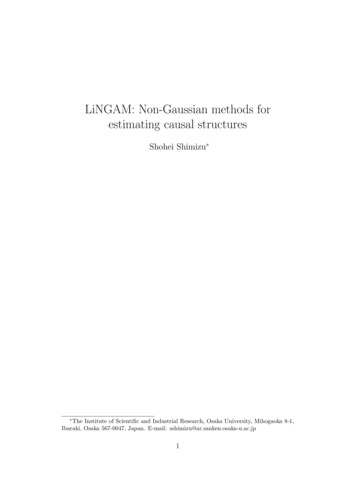
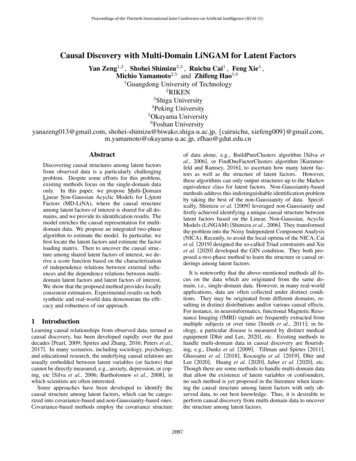
Proceedings of the Thirtieth International Joint Conference on Artificial Intelligence (IJCAI-21)4Average Variable Inflation Factors (VIF) are defined as the average VIF for all 100 independent trials of each range of weights.2101.21000 2000sample sizes.8.6.42345multicollinearity.64F1 scores.6.4.2500 1000 20005number of domains(g) Re. with Mul.100sample sizes200500 1000 2000sample sizes(c) F1. with .8(e) Pre. with Co.93200.8.26(d) Re. with Co.2100LiNANICATriad.8(b) Pre. with Sa.3We generated the data according to Eq.(1). Unless specified,each structure in a domain has 5 latent factors and each factor has 2 pure measurement variables with sample size 1000.See SM G.1 for the details. We compared our LiNA withNICA [Shimizu et al., 2009] and Triad [Cai et al., 2019]for single-domain data. Since NICA and Triad do not focus on multi-domain data, we used our method that did notconduct line 6 of Algorithm 1 as the comparison (MD*). Wedid experiments with i) different sample sizes; ii) highlycorrelated latent variables; iii) different numbers of latentfactors and iv) multi-domain data. For other robustness performances, please see SM G.2.i) Different sample sizes n 100, 200, 500, 1000, 2000,to verify the capability in small-sample-size schemes. In Figure 2(a)-(c), we found our LiNA has the best performance, especially with smaller sample sizes. As sample sizes decrease,performances of other methods decrease whereas LiNA remains incredibly preponderant. Although Triad’s recall iscomparable to ours with enough sample sizes, its precisionis the worst. The reason may be the sample sizes are not adequate to prune the directions, producing redundant edges.ii) Highly-correlated variables through different effectsof latent factors [ i, 0.5] [0.5, i], i 2,., 6. Their corresponding average Variable Inflation Factors (VIF) 4 are 22%,47%, 69%, 78% and 84%, respectively, which measure themulticollinearity of variables and higher VIFs mean the heavier multicollinearity. In Figure 2(d)-(f), we found that as VIFincreases, the accuracy of all methods declines in differentdegrees, but our method still outperforms the other comparisons, due to the employment of the elastic net regularization.iii) Different numbers of latent factors q 2, 3, 5, 10,to emphasize the capability of estimating causal effects, compared with NICA (Triad is not compared since it does not estimate effects). We applied the same method, CFA, to estimateĜ as the NICA. Overall, in Figure 3, we found LiNA givesbetter performances in all cases. The accuracy decreasesalong with more latent factors. Specifically, NICA is comparable to ours when q 2. However, as q 10, accuraciesboth decrease, but LiNA decreases much more slowly than.4F1 scoresrecallsprecisions5001recallsSynthetic Data200(a) Re. with Sa.2We performed experiments on synthetic and real data, including multi-domain and single-domain ones. Due to the unstable performance of Triad, we assume the structure in measurement models is known a priori for all methods.5.1.2100.62345multicollinearity6(f) F1. with Co.9.9F1 ng the identification results of LiNA/MD-LiNA, wepresent Theorems 2 and 3 to ensure that with our methods,asymptotically the resulting estimators Ḡ and H will be consistent to the true ones, while B̃ will be locally consistent toits DAG solution. The proofs are shown in SM C.3 and C.4.1.8recalls , then under conditions given in C0-C5 (see SM C.4), ourmethod using QPM with Eq.(7), is consistent to learn Ḡ andH, and locally consistent to learn B̃.6.32345number of domains(h) Pre. with Mul.MD(2)MD*(2).6MD(3)MD*(3).3MD(5)2345number of domainsMD*(5)(i) F1. with Mul.Figure 2: The recall (Re.), precision (Pre.) and F1 scores (F1.) of therecovered causal graphs between latent factors with different sample sizes (Sa.) i.e., n 100, 200, 500, 1000, 2000 in (a), (b) and(c), whose noises of latent factors follow Laplace distributions; withdifferent levels of multicollinearities (Co.) in (d), (e) and (f). Inparticular, in the x-axis, levels of multicollinearities of i 2, ., 6are 22%, 47%, 69%, 78% and 84%, repectively, in the average VIF;and with different numbers of domains (Mul.) in (g), (h) and (i).Solid lines are from our MD-LiNA while dotted lines are from thecomparison MD*. Higher F1 score represents higher accuracy.NICA. The reasons may be 1) more measurement variableswith the fixed sample size results in reduced power of CFAto estimate Ĝ, propagating errors to learn B̂; 2) the sparsityconstraint deals with small sample sizes while NICA doesnot. And NICA does not estimate the causal directions andeffects simultaneously, which may lack statistical efficiency.iv) Multi-domain data M 2, 3, 4, 5, through varyingnoises ε’s distributions (sub-Gaussian or super-Gaussian). Toobtain the true graph for evaluation, we generated the identical graphs of latent factors in each domain. We varied thenumber of latent factors, qm 2, 3, 5. In Figure 2(g)-(i), wefound F1 scores of both methods tend to decrease with moredomains or more latent factors increases. Specifically, in allcases MD-LiNA gives a better performance compared withMD*, in that MD* did neglect the problem that factors fromdifferent domains are represented by which factors of interest. Further, though we experimented with only qm 2, 3, 5,the whole causal graph is much more complicated, which hastotally M qm latent factors and 2M qm observed variables.5.2Real-World ApplicationsYahoo stock indices dataset. We aimed to find the causalstructure between different regions of the world, i.e., Asia,Europe, and the USA, each of which consisted of 2/3stock indices. They were Asia : {N225, 000001.SS} fromJapan and China, Europe : {BUK100P, FCHI, N100}from United Kingdom, France, and other European countries,

Proceedings of the Thirtieth International Joint Conference on Artificial Intelligence (IJCAI-21)-2-2-2-101Generating G2(a) G (q 2)4-1Eur.-2-2-101Generating B2(b) BLiNA (q 2)-2-101Generating BBUK100P Asia GSPC4BUK100P Asia GSPC01.85Eur.USAFCHI N100 NYA DJI(c) BNICA (q 2)10-1-2-101Generating GFCHI N100 NYA DJI-101Generating B-2-101Generating G10-12(g) G (q 5)-101Generating B-2-101Generating G(j) G (q A1(b)(c)Figure 5: Causal structures of fMRI hippocampus data using (a)LiNA, (b) NICA, and (c) Triad methods. Note that Triad output anempty graph, which implied all brain regions are independent witheach other. Solid blue lines are consistent edges with the anatomicalconnectivity while densely dotted red lines are spurious. Looselydotted blue lines represent redundant edges.-1-101Generating B2210-1-2-2Sub(a)(i) BNICA (q 5)Estimated B̂Estimated B̂-1PHC0-220212(h) BLiNA (q 5)11-2-2202-2-2-1Generating B(f) BNICA (q 3)Estimated B̂Estimated B̂-10-1-220Figure 4: Estimated stock indices networks using the (a) MD-LiNAand (b) MD* methods. Solid blue lines denote consistent edges withthe ground truth while densely dotted red lines are not.12(e) BLiNA (q 3)1(b)-2-22Estimated Ĝ0-12(d) G (q 3)Estimated Ĝ1-2-2USA2Estimated B̂Estimated B̂Estimated Estimated B̂1000001.SS28Estimated B̂20.2Estimated Ĝ210-1-2-2-101Generating B2(k) BLiNA (q 10)-2-101Generating B2(l) BNICA (q 10)Figure 3: Scatter plots of estimated causal structures versus the trueones with different numbers of latent factors q. Note that estimatesoutside the interval [-2,2] are plotted at the edges of this interval.(a), (d), (g) and (j) are scatter plots of the estimated factor loadingmatrix versus the true ones. (b), (e), (h) and (k) are scatter plots ofour method’s estimated adjacency matrix versus the true ones while(c), (f), (i) and (l) are of NICA method’s estimated matrix. The xaxis is the generating G or B while the y-axis is the estimated Ĝ orB̂. Closer to the main diagonal means higher accuracy.and USA : {DJI, GSPC, NYA} from the United States.We divided the data into two non-overlapping time segmentssuch that their distributions varied across segments and areviewed as two different domains. We tested its multicollinearity and used 10-fold cross validation to select parameter values. Details are in SM H.1. Due to the different timezones, it is expected the ground truth is Asia Europe USA [Janzing et al., 2010; Chen et al., 2014], with which ourrecovered causal structure in Figure 4 was in accordance.fMRI hippocampus dataset. We investigated causal relations between six brain regions of an individual: perirhinal cortex (PRC), parahippocampal cortex (PHC), entorhinal cortex (ERC), subiculum (Sub), CA1, and CA3/Dentate2102Gyrus (DG), each of which had left and right sides and weretreated as measurements [Poldrack et al., 2015]. We used theanatomical connectivity between regions as a reference forevaluation [Bird and Burgess, 2008; Ghassami et al., 2018].From Figure 5, we see though our method estimated one moreredundant edge, we obtained more consistent as well as lessspurious edges than NICA, while Triad failed to learn the relations between these regions in thi

Models (LiNGAM) [Shimizu et al., 2006]. They transformed the problem into the Noisy Independent Component Analysis (NICA). Recently, to avoid the local optima of the NICA, Cai et al. [2019] designed the so-called Triad constraints and Xie et al. [2020] developed the GIN condition. They both pro-posed a two-phase method to learn the structure or .