Transcription
Introduction to GIS using ESRI ArcGIS DesktopBefore you beginOutside of workshop: general GIS resources at MIT are available at libguides.mit.edu/gis.You will need an MIT Geodata Repository Account before beginning this exercise. If you do not alreadyhave an account, you can create one (libguides.mit.edu/content.php?pid 347508&sid 2843929). Clickon Create a User Account on the left-hand side of the page. Choose MIT Kerberos Account (or MIT webcertificate) as your account provider and select “Do not remember selection”. Click Continue. Log inusing your Kerberos username and password. This will bring you to the MIT Geodata Repository Accountcreation page where you can set your password.Before you begin, think about where you will be storing all the GIS files that you will be downloading andcreating in this exercise. You can create a working folder on the desktop or in the Documents folder onthe local C Drive on the computer you are using.IntroductionThis exercise is intended to introduce you to the basic use of ArcGIS for Desktop 10.1, a large programwith many extensions, tools and uses. In this workshop we will become familiar with the standard toolsin ArcMap used for creating and navigating maps and utilizing and analyzing the tabular informationbehind the maps. You will learn to: Find and add data from:o the MIT geodata repository, using: GeoWeb - a web browser interface which allows you to search for anddownload geospatial data from MIT and other partner repositories. A tool built at MIT to run on top of the ArcMap, ArcGIS interface; allows you toview and directly add MIT data to your ArcMap GIS project.o ESRI Resource Center through ArcGISo local media (CDROM, hard drive, etc)Symbolize vector dataAutomatically label data in the mapFind specific records of information and zoom directly to themSelect records that fall within the same geography as another—“spatial selection” or Select byLocationSubset data: export selected records to a new fileSelect by attributes (records in a table)Symbolize data by different fields in the attribute table: graduated colors and normalizingCreate a new field in the attribute table and calculate values in itJoin tabular data to a gis layer for display in the mapSymbolize multiple fields from the attribute table simultaneously using bar columns for display
Use the layout view to create a finalized map and export it in different formats (tiff, jpg, pdf, ai,etc.)Use ArcGlobe to look at your data in a form similar to Google EarthStarting out1. Open ArcMap (Start (Windows Icon in Lower Left Corner of Screen) All Programs ArcGIS ArcMap 10.1)You will be prompted on whether you want to open a new map project, or an existing one. You shouldopen a new map by selecting a “blank map” and clicking OK.
All of the controls are dockable. You can also click on the thumbtack symbolto “pin” a window, suchas the Table of Contents” to the screen or “unpin” it so that it hides off to the side when you’re notusing it. In this picture the tools panel, which has the pan and zoom tools,drag it away from the other tools, or snap it to any side of the window.is docked. You can2. In the top grey area of tools you can right click to see a list of additional tools you can easily turnon or off. If it is not already turned on, add the MIT Geodata Search Toolbar, as this will be usedin the following section. You will find many options within ArcGIS by right clicking on differentparts of the interface.What's on the interface, besides the pan and zoom tools? Various menus which give you access tocustomizing tools and map management tools. We will use many of these in the course of this tutorial.Find and add data from the MIT Geodata Repository: ArcMap toolbarThe MIT Geodata Repository provides a toolbar to search for geospatial data hosted by MIT using eitherkeywords or a geographical area. The geographical area search, labeled "Search Map Area" enables oneto zoom to an area on the map and look for all data that is in that area (without worrying about spelling,typos, foreign languages characters, or using correct descriptive terms).
1. Using the MIT Geodata Toolbar, click “Search metadata.” If you don’t yet have an account, clickon “No Account? Register Now.” and follow the instructions at the beginning of this exercise.2. Once logged in, type “boston” (the search is not case sensitive) into the search for box and click“search”3. Select the “BRA Planning Districts, 2000” layer and click “Add Selected Layer to Map”.4. Scroll down and select the “Land parcels, 2006” layer, click “View Metadata”1 to see thedescriptive information in a web browser, then add the layer.5. Scroll down and add the “Open Space, 1999” layer.6. Exit the MIT Geodata Repository Search Results dialog box.7. In the Table of Contents of ArcGIS (where all 3 layer names are listed) turn the layers on or offwith the checkboxes located to the left of each layer name. Leave the parcel layer unchecked fornow so that the next few steps will go more quickly (layers with many small records take longerto draw). If things are taking a while to refresh, you can press Esc to stop the refresh.8. Adjust which layer draws on top by adjusting the order in which they are displayed in the TableOf Contents (click and drag a layer name above or below another layer). You will want your openspace/parks layer on top so it won’t be covered by the BRA planning districts polygon.9. Right click on the parcels layer and click Open Attribute Table. Every point, line, or polygon filehas an attribute table. This table can have many columns, such as the one you are looking atnow. Any data in the attribute table can be used for displaying and labeling on the map andmaking queries. You can also create new columns in the table to add data or calculations to it.Metadata can be key to understanding attribute tables that use codes and abbreviations, suchas this table. Close the attribute table.1Metadata describes where the data came from, what can be found within it, when it was created, etc. The onlinelinkage also has a link to the MIT Libraries Barton catalog record, which notes that this data is also available on CDin the GIS Lab, Rotch Library. The metadata also explains that the file you are viewing from the MIT GeodataRepository was created by joining a numeric property parcel table with a GIS file representing parcels as polygons.Since there can be multiple units within one parcel polygon (e.g. condominiums) not all records in the originalproperty parcel table are included in this GIS file. If a person wants all numeric property parcel data included in theoriginal table, they would need to come into the library and use the CD.
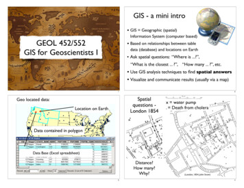
Find and add data from the MIT Geodata Repository: GeoWeb1. There is a link to GeoWeb from the MIT GIS Services homepage, or you can navigate directly toGeoWeb at web.mit.edu/geoweb. The website works best using Google Chrome or MozillaFirefox.If you do not have MIT personal certificates installed in your web browser then you will see a messagethat asks you to log in using your MIT certificates or Touchstone. For this exercise you will be using adataset that is publicly accessible, so it is not necessary that you log in.GeoWeb provides a Getting Started tab and a user guide so you can learn more about it, how it works,and what you can expect to find in it. The front page of GeoWeb looks like this:GeoWeb uses Google Maps as a background layer and OpenLayers for controlling the map interface. Youcan use the navigation tools, similar to what you find in Google maps, for zooming and panning in themap.Click the Search tab near the top left portion of the page to begin searching for geospatial data. Notethat the “Limit results to visible map area” is checked by default.
1. Before searching for any particular keywords, use Find Place, in the top right corner of the map,to help locate and zoom in to a particular location on the map. Type “Boston, MA” and click go.The map should reload around Boston.2. You can also press shift and use the mouse to draw a box around the area of interest and searchwhat falls within it.Your search results (approximately 1,824) appear in the Search tab. To see the metadata of any layer,click thebutton. Checking the box in the preview column will draw the layer on the map. You canselect as many layers as you like to draw on the map.3. In the Search tab, search for “subway” and preview the Boston, MA (MBTA Subway Lines, 2006)layer that appears in the results.There are a variety of controls here that let you reorder the layers you have selected to draw, makethem display or not, look at the attribute table information, change the opacity, and more. GeoWeb isnot a GIS. It is a tool for easily finding, viewing, and accessing GIS data held in the MIT GeodataRepository or other partner repositories. Check the box in the cart columnfor the MBTA SubwayLines layer and click on the Cart tab in the upper left corner. From here you can download the data in avariety of formats, including shapefile for use in ArcGIS and KML/KMZ for use in Google Earth. However,instead of downloading the data, for this exercise we are going to use a different method to use the datain ArcMap.In the cart, the "Share" button lets one easily save a link to the data layers in the cart for later use or forsharing with a partner. This link also lets any member of the MIT community with ArcGIS installed easilytake MIT data discovered in GeoWeb directly into ArcMap, where there are many tools for working withthe data and creating maps. Please note that the link only allow you to add MIT-owned data directlyinto ArcMap. When browsing non-MIT layers within Geoweb, you must download them directly ontoyour computer before using them in ArcMap.
4. Click the “Share” button and select and copy the link web address.5. Return to ArcMap and click “Data from GeoWeb” on the MIT Geodata search toolbar. Paste thelink and click Add Layers. The MBTA subway lines should now appear on your map.Add a basemap from ArcGIS Online1. Click the dropdown arrow next to the add data button (2. Select “Add basemap”).
3. Click on imagery and click add. If you get a Geographic Coordinate Systems warning, click close.This happens because the imagery file from ESRI is using a different coordinate system and projectionthan the other data layers you previously brought into ArcMap. This means ArcGIS will be performingcalculations in the background to make the data line up. You do not need to worry about this in thisexercise, so just click close. If you are working on a project in the future where spatial accuracy isimportant then you may want to perform the extra steps to get all your data into one preferredprojection and coordinate system.Note that the layer is served over the web so it may take some time to draw (and that you have to beconnected to the internet for it to continue drawing). Also what you see depends on the scale you areworking in on your map - as you zoom in closer you will typically find more detailed information. Yourscale is displayed in the Standard toolbar and automatically adjusts as you zoom in and out.
4. You may want to uncheck the basemap layer (under the Table of Contents) to improveperformance as you continue working through the exercise.Symbolize vector dataMake the parks display as green1. Right click the polygon below the open space/parks layer(sde data.us ma boston g52parks 1999) and change the color to greenSymbolize the planning layer by name and label the neighborhoods2. Right click the Boston Planning Districts layer name (sde data.us ma boston g45plnng 2000)and choose properties. This will bring up the Layer Properties window.3. Click the symbology tab.4. Change the symbology to Categories: Unique values and select "NAME" in the Value Field.5. Click “Add All Values”, and click “Apply”.6. In the Labels tab, check “Label features in this layer”, and make sure the Label Field is “NAME”.Click OK. Alternatively you could right click on the planning layer name and click 'Label Features'to label the map without opening the properties window. Anything in your attribute table canbe easily used for labeling.7. Save your map document to the desktop or a working folder on your local drive using File, Save(you will learn more about saving later in the exercise).
Find Back Bay and zoom to it1. Click the binoculars on the main toolbar, and choose the Features tab.2. In the Find box, type “Back Bay”.3. In the In box, limit the search to sde data.us ma boston g45plnng 2000, and click the Findbutton.4. Right click the result of the find, and choose “Select”. This will select the Back Bay/BeaconHill polygon and turn its outline blue on your map.5. Right click the result of the find again, and click “Zoom to”. Close the Find window6. Once you are zoomed to Back Bay, set the parcel file to display by checking the box to the left ofthe layer named sde data.us ma boston g47parcels 2006.
Select all the parcels within Back Bay (Select by Location)1. In the Selection menu at the top, click “Select By Location”.2. Use the following parameters:a. Selection method: Select features fromb. Target layers: parcelsc. Source layer is boston planning districts (sde data.us ma boston g45plnng 2000)d. Make sure use selected features is checkede. Spatial selection method: “Target layer(s) features are within the Source layer feature”.f. In other words, select parcels that are within the selected neighborhood. Click OK.
Export the Back Bay parcels to a new, smaller fileWe are going to export the selected parcels in Back Bay into a new, smaller file. Exporting the data ofinterest is typically the easiest way to subset a dataset to only the desired records and keep your filesizes smaller and more manageable.1. Right click the parcels layer, select Data Export Data.
2. Export the “selected features” using the same coordinate system as the layer’s source data intoyour working folder and name the file parcels.shp. Note that file names and locations can bevery important when working on projects. Users tend to generate many files when working onGIS projects, so you want to make sure to use file names that are descriptive and easy toremember in the future. If you exporting your data to a drive you have never before used inArcGIS, you may not see it listed. In this case, use the Connect To Folder button ( ) to add thedrive.If you are having trouble saving the layer:a. Click on the folder icon to view and edit the save location.b. Make sure that the “save as type” is set to “shapefile” not “file and personal geodatabasesfeature classes”3. Click Save and then click Yes when asked if you want to add the exported data to the map as alayer.4. Turn off the old parcels layer.
5. Clear the selected features by clicking the “clear selected features” button in the top menu bar( ).6. Save your map document.Select by attributes to explore gross tax in the parcels layer1. Right click parcels and choose “Open Attribute Table”. Quickly look through the many fields inthis file. You could look up the codes for fields like LU (Land Use) in the metadata.2. Right click the GROSS TAX column, and select “Statistics”.3. What is the mean gross tax for all parcels in Back Bay? ( 45,292)4. Close the statistics dialog box, and click the Select By Attributes button ( ) at the top of thetable window.5. Create a new selection where GROSS TAX (double click in the list) 0 (in the dialog box). ClickApply.6. In the bottom of the table, change from all to selected records () so you have fewer recordsto scroll through.Explore other queries with GROSS TAX and the statistics button to find out:7. How many parcels in Back Bay list a gross tax of 0? (1,052) Who owns them?You can switch the selection using the button ( ) at the top of the table. This will select all the recordswhere the gross tax is not equal to 0. View only these selected records.8. What is the smallest gross tax paid that is greater than zero? ( 4)9. What is the greatest amount of gross tax paid in Back Bay? ( 18,296,555)
10. What is the mean tax paid for all records with a gross tax greater than 0? ( 70,238)11. Close the attribute table and clear the selection using the button ( ) in the toolbar.Symbolize according to total land value (graduated colors and normalizing)1. Right click the parcels layer and choose “Properties”.2. In the symbology tab, change the symbology to “Quantities: Graduated colors” withFY2006 TOT as the value and no normalization. Normalizing is the same as using a different fieldin the denominator. You could normalize by gross area to get the cost per square foot. In thenext section we will create a new field with the cost per square foot, so the values will bepermanently stored in the file.3. Choose a Color Ramp that is clearly going from low to high. Experiment with the number ofclasses and classification type and choose the one that seems best. The classification type canonly be changed by clicking the “Classify ” button. Click OK to close the layer propertieswindow.4. Right click the file name and click “Save As Layer File” to save your symbology to a file. Whenyou save your symbology to a layer file you can re-apply the symbology after trying others and italso gives you the option to apply the same symbology to other files. This layer file only saves
the symbology, not the data. If you move your files around you must be sure to move all files,not just the project or layer files.5. Save your map document.Calculate the cost per square foot1. Right click the parcels layer and open the attribute table.2. Add a field by clicking the Options buttonand selecting Add Field.3. Name your field “cost sf” (there is a 10 character limit on field names) and change the type toShort Integer. Click OK.4. Click “Select By Attributes” at the top of the table and create a new selection where“GROSS AREA” 0. Click apply. Some of the Gross Area records have a zero value, which wouldcause an error message since you can’t divide by zero. Selecting everything in Gross Areagreater than zero will make the next calculation perform only on the selected records.5. Scroll all the way to the right in your attribute table, right click on the cost sf heading, andchoose “Field Calculator”. If asked if you want to perform the action outside an editing session,click “Yes”6. Create an expression where [FY2006 TOT] / [GROSS AREA] by double clicking on those fieldsand click OK.7. Right click on cost sf and choose “Sort Descending” to make the most expensive homes persquare foot list at the top of your table.8. Right click on cost sf and choose “Statistics” to look at the min, max, median, etc.
9. Clear the selection using the button in the top toolbar of the table window and exit out of theattribute table.10. Save your map document.Thematic mapping: Explore cost per square foot1. Right click on the parcels layer, click Properties, and navigate to the Symbology tab.2. Change the value to cost sf and change the number of classes from the default of 5 to 10. ClickApply and look at the map.3. Click Classify and change the classification method from the default of Natural Breaks (Jenks) toEqual Interval. Click OK, and then Apply.Explore the other classification types and notice how they change the look of the map. Natural breaks: Intervals are broken out based on natural clusterings of data.
Equal interval: The range of possible values is divided into equal-sized intervals. Because thereare usually fewer observations at the extremes, the number of values is less in the extremeclasses. This option is useful to highlight changes in the extremes. It is probably best applied tofamiliar data ranges such as percentages or temperature.Quantile - The range of possible values is divided into unequal-sized intervals so that thenumber of values is the same in each class. Classes at the extremes and middle have the samenumber of values. Because the intervals are generally wider at the extremes, this option isuseful to highlight changes in the middle values of the distribution.Map symbology can be used to alter the way people view and understand information, just likestatistics. It is important to understand what you want to express in your map and how to bestsymbolize your data.Add data to ArcMap from a driveYou will need to download some of the data used in the remainder of this exercise. If you are using aDIRC computer, the data is available within the IntroExerciseData.zip file located inT:\Intro GIS IAP2013Please copy the zip file to your working folder before unzipping. Alternatively, you can download thedata on the MIT GIS website: http://libguides.mit.edu/content.php?pid 347508&sid 2844939 (lookunder the Introduction to GIS section of the page).1. Use the Add Data button in the top of the toolbar to add census blocks.shp andcen2k b pop age gen.dbf to your map document.
If you are adding data from a drive you have never before used, you may not see it listed. In this case,use the Connect To Folder button ( ) to add the drive. To add more than one piece of data at the sametime, hold the Ctrl key as you select the layers.Notice that your Table Of Contents changes when you add the .dbf (database) file. It has automaticallyswitched to the Source view, which organizes the datasets according to where they are located on yourdrives. Notice that the cen2k b pop age gen.dbf is there, but cannot be displayed on the map since itis only a data table and contains no spatial information. Switch back to the Display view by clicking onthe “List By Drawing Order” button ( ) at the top of the Table Of Contents. Notice that thecen2k b pop age gen.dbf is no longer listed, since it is not part of the map display, but it is availablefor use in your project.2. Right click census blocks.shp and open the attribute table to explore the fields.3. Switch back to the “List by Source View”in the Table Of Contents. Right clickcen2k b pop age gen.dbf and click open to view the attribute table and explore the fields.These files are of gender by age group in tabular form and a US census block (2000) shapefile from theMassGIS website (www.mass.gov/mgis/laylist.htm). You can use them to explore if the number of malesand females is fairly equal between different census blocks in Back Bay. The MassGIS website stated that“the following table, available in dBase format (.dbf), which provides detailed demographicsinformation, may be joined to the Blocks shapefiles on the LOGRECNO item.” If you want a fuller set ofvariables to choose from the US Census, you should use these other sources: US Census Bureau (factfinder2.census.gov/): American Factfinder search is a way to find datasuch as population and average income.Geolytics: a company that has repackaged US Census data and made it easier to map. The MITLibraries have an assortment of Geolytics programs, which can be found using Barton and doingan advanced search where publisher Geolytics. All Geolytics programs in the MIT Librariescollection are loaded on the Census workstation in the GIS lab.MIT Libraries Census guide (libguides.mit.edu/content.php?pid 347508&sid 3386296)summarizes a lot of information: what's in the census, how it's broken down, how to map it, etcMIT Libraries Social Science Data Services (libraries.mit.edu/guides/subjects/data)
Join tabular data to a shapefile1. Right click the name of the file TO which you want to join the data (census blocks.shp), andselect Joins And Relates Join2. Join attributes from a table. The join will be based on LOGRECNO in this layer. The table towhich you’re joining this layer is cen2k b pop age gen, and the join is based on the field of thesame name in this table. Click OK.3. You will be asked if you want to index the join field in order to improve performance. Since ourfile does not have many records performance will not be noticeably increased, so click No.4. Open the census blocks attribute table by right clicking and notice the column names now beginwith the table name (if you don’t see this, you may need to turn off “Show Field Aliases” in theoptions menu of the attribute table). A join matches exact records one-to-one, and is not
permanent unless a new file is created by exporting. Also, the field names are too long to read inthe symbology options with this naming format.5. Right click census blocks then go to Data Export data. Export the joined file to a new filenamed block demog.shp in a local drive or on the desktop.6. Save your map document.Symbolizing multiple fields in a shapefile using bar columns1. Right click the block demog layer and select properties.2. Under the symbology tab, change the symbology of block demog.shp to Charts Bar/Column3. Select pop male and pop fem for display and give each a color that will be easy to rememberand distinguish.Do most blocks have a fairly even number of males and females?Create a layout of your map ready for publishing1. On the main toolbar menu at the top of ArcMap click View Layout View.2. Change your map from portrait to landscape (File Page and Print Setup).3. Click on any part of your map using the arrow tool. Adjust the data frame (area in dotted bluelines) to fill most of the page (area in the light gray box) but leave room for a title, scale bar, etc.4. On the main toolbar click Insert Title, and choose a title.5. Insert a legend using the same menu, include the appropriate layers you want in your legend,click next until you complete the legend dialog screens, and arrange the legend on your page soit fits with the map.6. Insert a North arrow in the same menu, and choose one of the many options.7. Right click in your toolbar area and turn on the Data Frame Tools. Rotate your data frame sothat the Charles River looks horizontal on your page. Note that your north arrow automaticallyrotates as you rotate your data frame.8. Insert a scale bar using the insert menu, and choose one of the many scale bars.9. Right click the scale bar and choose Properties. Click the Scale and Units, and set your divisionunits to kilometers. You can also change the label to “km” to save space.10. Insert a text box to add your name, date, and sources for your data. You can also insert a largervariety of textboxes that allow you to change their background color, by using the “draw”toolbar (right click in the toolbar and select it if it is not currently displayed).11. Change the scale of your map by zooming in or out or typing in a desired scale in the top toolbarand notice the scale bar automatically updates.Export your map to a pdf file1. Click File Export Map2. Choose PDF in “Save as type”.
Note that if you save as an AI (Adobe Illustrator), the layers will remain as separate, editable layers inIllustrator. If you save as JPEG or TIFF, you can adjust the resolution of the exported file.3. Open your map in Adobe Acrobat to see what it looks like.Save your ArcMap Document1. Click File Save from the top menu bar.Note that when you save an ArcMap document, you are only saving a link to the layers in your project. Ifyou move your project to a new location, you will need to move all the files linked to your project withit. Each shapefile has multiple files associated together, and they need to stay together to workproperly!By default, ArcMap stores the full path name to each layer in the ArcMap document. This means that ifyou move your files around, your path name will change and you will need to redirect ArcMap to thenew file location for each folder of data. If you will be moving files around, it is recommended that yousave a virtual path to the data files in your project.2. Go to File Map Document Properties, and check the “Store relative pathnames to datasources” box.Creating a Map Package for sharingAs noted above, when you save an ArcMap document, only the link to the layers is saved, not the layersthemselves. If you will be sharing your maps or accessing them from another location, you can save yourmap document as a map package.A map package contains a map document (.mxd) and the data referenced by the layers it contains,packaged into one convenient, portable file. Map packages can be used for easy sharing of mapsbetween colleagues in a work group, across departments in an organization, or with any other ArcGISusers via ArcGIS online. Map packages have other uses, too, such as the ability to create an archive of aparticular map that contains a snapshot of the current state of the data used in the map.1. Click File Share As Map Package on the main menu. This will open the Map Package dialogbox.
2. Name your new map package3. Specify where to save your map package - either as a file on disk or in your ArcGIS onlineaccount. For this exercise, save the map on your working folder. In the future, you can create anArcGIS online account if you wish. Add an item description, tags, and summary using the “ItemDescription” tab.4. Click Analyze to analyze your map for any errors or issues. You must analyze before you cansave it to disk or share it to ArcGIS online. If any issues are discovered, a Prepare window willappear with a list of issues. Right-click on each Prepare message to get more information, readhelp for the error, and to click on suggested fixes.5. Once validated, the Share button will be enabled. Click Share to create your map package.Using ArcGlobe to look at your data (similar to Google Earth)1. Open ArcGlobe (Start All Programs ArcGIS ArcGlobe 10.1).2. Click the “Add Data” button on the top toolbar and add your parcels.shp data to the map. Thisopens an import wizard. Choose a “Typical Scale” by dragging the marker until the city blocksare indicated, about 1:610. Click Next and Finish to close the wizard. Ignore any warning aboutmismatched projections.3. Move the parcels layer to the top of the “Draped layers” category and right click the layer andselect “Zoo
Use the layout view to create a finalized map and export it in different formats (tiff, jpg, pdf, ai, etc.) Use ArcGlobe to look at your data in a form similar to Google Earth Starting out 1. Open ArcMap (Start (Windows Icon in Lower Left Corner of Screen) All Programs ArcGIS ArcMap 10.1)