Transcription
A Mathematical Introduction toTraffic Flow TheoryBenjamin Seibold (Temple University)Flow rate curve for LWR modelsensor dataflow rate function Q(ρ)Flow rate Q (veh/sec)32100density ρρmaxSeptember 9–11, 2015Tutorials Traffic FlowInstitute for Pure and Applied Mathematics, UCLABenjamin Seibold (Temple University)Mathematical Intro to Traffic Flow Theory09/09–11/2015, IPAM Tutorials1 / 69
References for Further ReadingSome References for Further Readinggeneral: wikipedia (can be used for almost every technical term)traffic flow theory: wikibooks, “Fundamentals of Transportation/Traffic Flow”;Hall, “Traffic Stream Characteristics”; Immers, Logghe, “Traffic Flow Theory”traffic models: review papers by Bellomo, Dogbe, Helbingtraffic phase theory: papers by Kerner, et al.optimal velocity models and follow-the-leader models: papers by Bando,Hesebem, Nakayama, Shibata, Sugiyama, Gazis, Herman, Rothery, Helbing, et al.connections between micro and macro models: papers by Aw, Klar, Materne,Rascle, Greenberg, et al.first-order macroscopic models: papers by Lighthill, Whitham, Richards, et al.second-order macroscopic models: papers by Whitham, Payne, Aw, Rascle,Zhang, Greenberg, Helbing, et al.cellular models and cell transmission models: papers by Nagel, Schreckenberg,Daganzo, et al.numerical methods for hyperbolic conservation laws: books by LeVequetraffic networks: papers by Holden, Risebro, Piccoli, Herty, Klar, Rascle, et al.Benjamin Seibold (Temple University)Mathematical Intro to Traffic Flow Theory09/09–11/2015, IPAM Tutorials2 / 69
References for Further ReadingOverview1Fundamentals of Traffic Flow Theory2Traffic Models — An Overview3The Lighthill-Whitham-Richards Model4Second-Order Macroscopic Models5Finite Volume and Cell-Transmission Models6Traffic Networks7Microscopic Traffic ModelsBenjamin Seibold (Temple University)Mathematical Intro to Traffic Flow Theory09/09–11/2015, IPAM Tutorials3 / 69
Fundamentals of Traffic Flow TheoryOverview1Fundamentals of Traffic Flow Theory2Traffic Models — An Overview3The Lighthill-Whitham-Richards Model4Second-Order Macroscopic Models5Finite Volume and Cell-Transmission Models6Traffic Networks7Microscopic Traffic ModelsBenjamin Seibold (Temple University)Mathematical Intro to Traffic Flow Theory09/09–11/2015, IPAM Tutorials4 / 69
Fundamentals of Traffic Flow TheoryWhat do we mean by “Traffic Flow”?Two extreme situations: traffic flow modeling trivial/easyVery low densityNegligible interaction between vehicles;everyone travels their desired speedBenjamin Seibold (Temple University)(Almost) complete stoppageFlow dynamics irrelevant;simply queueing theoryMathematical Intro to Traffic Flow Theory09/09–11/2015, IPAM Tutorials5 / 69
Fundamentals of Traffic Flow TheoryWhat do we mean by “Traffic Flow”?Traffic flow modeling of importance, and challengingTraffic dense but movingMicro-dynamics: by which laws do vehicles interact with each other?Laws of flow, e.g.: how does vehicle density relate with flow rate?Macro-view: temporal evolution of traffic density? traffic waves? etc.Benjamin Seibold (Temple University)Mathematical Intro to Traffic Flow Theory09/09–11/2015, IPAM Tutorials6 / 69
Fundamentals of Traffic Flow TheoryFundamental QuantitiesUniform traffic flowdriving direction speed-vehicle length distance dSome fundamental quantities density ρ: number of vehicles per unit length (atfixed time) flow rate (throughput) f : number of vehiclespassing fixed position per unit time speed (velocity) u: distance traveled per unit time time headway ht : time between two vehicles passingfixed position space headway (spacing) hs : road length per vehicle occupancy b: percent of time a fixed position isoccupied by a vehicleBenjamin Seibold (Temple University)Mathematical Intro to Traffic Flow Theoryspacing hsRelationshs d ρ #lanes/hsf #lanes/htf ρuρmax #lanes/ ρ b · ρmaxetc.09/09–11/2015, IPAM Tutorials7 / 69
Fundamentals of Traffic Flow TheoryFundamental QuantitiesNon-uniform traffic flowdriving direction ------vehicles have different velocities pattern changesFundamental quantitiesKey questions density ρ: number of vehicles per unitlength (at fixed time) as before flow rate f : number of vehicles passingfixed position per unit time as before time mean speed: fixed position, averagevehicle speeds over time space mean speed: fixed time, averagespeeds over a space interval bulk velocity: u f /ρ usually meantin macroscopic perspective Given vehicle positions andvelocities, how do they evolve? Impossible to predict on level oftrajectories (microscopic). But it may be possible on levelof density and flow rate fields(macroscopic). Needed: connection betweenmicro and macro description.Benjamin Seibold (Temple University)Mathematical Intro to Traffic Flow Theory09/09–11/2015, IPAM Tutorials8 / 69
Fundamentals of Traffic Flow TheoryMicro vs. MacroMicroscopic descriptionindividual vehicletrajectoriesvehicle position: xj (t)vehicle velocity:dxẋj (t) dtj (t)acceleration: ẍj (t)Macroscopic descriptionfield quantities,defined everywhereMicro view distinguishes vehicles;macro view does not.vehicle density: ρ(x, t)velocity field: u(x, t)flow-rate field:f (x, t) ρ(x, t)u(x, t)Benjamin Seibold (Temple University)Traffic flow has intrinsic irreproducibility.No hope to describe/predict precise vehicletrajectories via models [also, privacyissues]. But, prediction of large-scale fieldquantities may be possible.Mathematical Intro to Traffic Flow Theory09/09–11/2015, IPAM Tutorials9 / 69
Fundamentals of Traffic Flow TheoryMicro vs. MacroMicroscopic macroscopic: “kernel density estimation” (KDE)Some approaches to go from x1 , x2 , . . . , xN to ρ(x):piecewise constant: let x1 x2 . . . , xN ; for xj x xj 1 , defineρ(x) 1/(xj 1 xj ).no unique density at vehicle positions;does not work for aggregated lanesmoving window: at position x, define ρ(x) as the number of vehiclesin [x h, x h], divided by the window width 2h.integer nature;discontinuous in timesmooth Pmoving kernels: each vehicle is a smeared Dirac delta;2ρ(x) j G (x xj ); use e.g. Gaussian kernels, G (x) Z 1 e (x/h) .Most KDE approaches require a length scale h that must be larger than the typicalvehicle distance, and smaller than the actual length scale of interest (road length).Macroscopic microscopic: “sampling”Some approaches to go from ρ(x) to x1 , x2 , . . . , xN :sampling via rejection, inverse transform, MCMC, Metropolis, Gibbs, etc.Benjamin Seibold (Temple University)Mathematical Intro to Traffic Flow Theory 09/09–11/2015, IPAM Tutorials10 / 69
Fundamentals of Traffic Flow TheoryContinuity EquationOnce we have a macroscopic (i.e. continuum) descriptionVehicle density function ρ(x, t); x position on road; t time.Number of vehicles between point a and b:Z bm(t) ρ(x, t)dxaTraffic flow rate (flux) is product of density ρ and vehicle velocity uf ρuChange of number of vehicles equals inflow f (a) minus outflow f (b)Z bZ bdm(t) ρt dx f (a) f (b) fx dxdtaaEquation holds for any choice of a and b:continuity equationρt (ρu)x 0 ρt fx 0Note: The continuity equation merely states that no vehicles are lost or created. Thereis no modeling in it. In particular, it is not a closed model (1 equation for 2 unknowns).Benjamin Seibold (Temple University)Mathematical Intro to Traffic Flow Theory 09/09–11/2015, IPAM Tutorials11 / 69
Fundamentals of Traffic Flow TheoryStochasticity of Traffic FlowA critical note on stochasticityIt is frequently stated that “traffic is stochastic”, or “traffic is random.”Or even further: “traffic flow cannot be described via deterministic models.”Problems with these statementsA stochastic description is only useful if one defines the random variables,and knows something about their (joint) probability distribution.Certain observables in a stochastic model may evolve deterministically. Itmatters what one is interested in: the evolution of real traffic flow may bereproduced quite well by a model, if one is interested in the density onlength scales much larger than the vehicle spacing. In turn, attempting tomodel the precise trajectories of the vehicles is most likely hopeless.A better formulation and research goalsTraffic has an intrinsic irreproducibility (that cannot be overcome, say, viamore a careful experiment), due to hidden variables (e.g. drivers’ moods).Goals: 1) find models that describe macroscopic variables as well as possible( fundamental insight into mechanics); 2) combine these models withfiltering to incorporate data ( prediction).Benjamin Seibold (Temple University)Mathematical Intro to Traffic Flow Theory 09/09–11/2015, IPAM Tutorials12 / 69
Fundamentals of Traffic Flow TheoryMeasurementsExamples of ways to measure traffic variableshuman in chair: count passing vehicles ( flow rate)single loop sensor: at fixed position, count passing vehicles (flow rate)and measure occupancy ( density and velocity indirectly, assumingaverage vehicle length)double loop sensor: as before, but also measure velocity directlyaerial imaging: photo of section of highway; direct measure of densityGPS: precise trajectories of a few vehicles on the roadobservers in the traffic stream: as GPS, but also information aboutnearby vehiclesprocessed camera data: precise trajectories of all vehicles (NGSIMdata set); perfect data, but not possible on large scaleInferring macroscopic variables (density, flow rate, etc.)Traditional means of data collection measure them (almost) directly.Modern data collection measures very different things. Inferringtraffic flow variables (everywhere and at all times) is a key challenge.Benjamin Seibold (Temple University)Mathematical Intro to Traffic Flow Theory 09/09–11/2015, IPAM Tutorials13 / 69
Fundamentals of Traffic Flow TheoryBruce Greenshields collecting data (1933)First Traffic Measurements and Fundamental DiagramDeduced relationshipu U(ρ) umax (1 ρ/ρmax ),ρmax 195 veh/mi; umax 43 mi/hFlow ratef Q(ρ) umax (ρ ρ2 /ρmax )Contemporary measurements (Q vs. ρ)Flow rate curve for LWRQ modelsensor dataflow rate function Q(ρ)3Postulated density–velocity relationshipFlow rate Q (veh/sec)[This was only 25 years after the first Ford Model T (1908)]2100density ρρmax[Fundamental Diagram of Traffic Flow]Benjamin Seibold (Temple University)Mathematical Intro to Traffic Flow Theory 09/09–11/2015, IPAM Tutorials14 / 69
Fundamentals of Traffic Flow TheoryFundamental Diagram (FD) oftraffic flow (sensor data)Flow rate curve for LWRQ modelsensor dataflow rate function Q(ρ)Flow rate Q (veh/sec)3Fundamental DiagramFascinating factFDs exhibit the same features, for highwayseverywhere in the world: f Q(ρ) for ρ small (free-flow) for ρ sufficiently large (congestion),FD becomes set-valued2 set-valued part: f decreases with ρ1[Greenshields Flux]00density ρρmaxFlow rate curve for LWR modelsensor dataflow rate function Q(ρ)Ideas and concepts ignore spread and define functionf Q(ρ), e.g.: Greenshields (quadratic),Daganzo-Newell (piecewise linear) fluxFlow rate Q (veh/sec)3 empirical classification and explanation traffic phase theory [Kerner 1996–2002]2 explanation of spread via “imperfections”:sensor noise, driver inhomogeneities, etc.1[(smoothed) Daganzo-Newell Flux]00density ρBenjamin Seibold (Temple University)ρmax study of models that reproduce spread(esp. second-order models)Mathematical Intro to Traffic Flow Theory 09/09–11/2015, IPAM Tutorials15 / 69
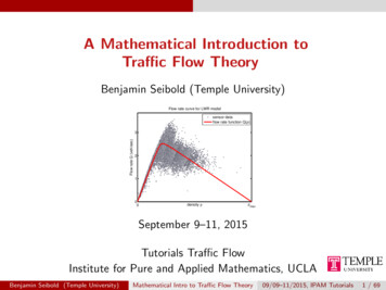
Fundamentals of Traffic Flow TheoryPhase transition induced by trafficwaves in macroscopic model[S, Flynn, Kasimov, Rosales, NHM 8(3):745–772, 2013]Traffic phase theory(here: 2 phases)[Kerner 1996–2002]sensor dataSy0.7nceonizedfloweflow0.5curvhr0.60.3flow rate Q: # vehicles / sec.0.8Freflow rate: # vehicles / lane / sec.0.90.4Fundamental Diagram0.2equilibrium curvesonic pointsjamiton linesjamiton envelopesmaximal jamitonssensor data0.80.60.40.20.1000.20.40.6density ρ / ρmax0.81000.20.40.6density ρ / ρmax0.81Also: 3-phase theory (wide moving jams)A key challenge in traffic flow theoryMany open questions in explaining (phenomenologically), modeling, andunderstanding the spread observed in FDs.Benjamin Seibold (Temple University)Mathematical Intro to Traffic Flow Theory 09/09–11/2015, IPAM Tutorials16 / 69
Traffic Models — An OverviewOverview1Fundamentals of Traffic Flow Theory2Traffic Models — An Overview3The Lighthill-Whitham-Richards Model4Second-Order Macroscopic Models5Finite Volume and Cell-Transmission Models6Traffic Networks7Microscopic Traffic ModelsBenjamin Seibold (Temple University)Mathematical Intro to Traffic Flow Theory 09/09–11/2015, IPAM Tutorials17 / 69
Traffic Models — An OverviewThe Point of ModelsOne can study traffic flow empirically, i.e., observe and classify what onesees and measures.So why study traffic models?Can remove/add specific effects (lane switching, driver/vehicleinhomogeneities, road conditions, etc.) understand which effectsplay which role.Can study effect of model parameters (driver aggressiveness, etc.).Can be analyzed theoretically (to a certain extent).Can use computational resources to simulate.Yield quantitative predictions ( traffic forecasting).We actually do not really know (exactly) how we drive. Models thatproduce correct emergent phenomena help us understand our drivingbehavior.Traffic models can be studied purely theoretically (mathematicalproperties). That is fun; but ultimately models must be validatedwith real data to investigate how well they reproduce real traffic flow.Benjamin Seibold (Temple University)Mathematical Intro to Traffic Flow Theory 09/09–11/2015, IPAM Tutorials18 / 69
Traffic Models — An OverviewMicroscopic modelsẍj G (xj 1 xj , uj , uj 1 )Types of Traffic ModelsMacroscopicmodels(ρt (ρu)xCellular models 0(u h)t u(u h)x τ1 (U u)1000900positions of vehicles x(t)8007006005004003002001000020406080100time t120140160180200IdeaDescribe behavior of individualvehicles (ODE system).Micro Macro macro limit of micro when#vehicles micro discretization ofmacro in LagrangianvariablesBenjamin Seibold (Temple University)Methodology and role Describe aggregate/bulkquantities via PDE. Natural framework formultiscale phenomena,traveling waves, and shocks. Great framework toincorporate sparse data[Mobile Millennium Project].IdeaCell-to-cell propagation(space-time-discrete).Cellular Macro macro limit of cellular when #cells cellular discretization of macro inEulerian variablesMathematical Intro to Traffic Flow Theory 09/09–11/2015, IPAM Tutorials19 / 69
Traffic Models — An OverviewMicroscopic Traffic ModelsMicroscopic Traffic Models — Typical SetupN Vehicles on the roadPosition of j-th vehicle: xjVelocity of j-th vehicle: vjAcceleration of j-th vehicle: ajPhysical principlesVelocity is rate of change ofposition: vj ẋjAcceleration is rate of changeof velocity: aj v̇j ẍjuse computersto solve Benjamin Seibold (Temple University)“Follow the leader” modelAccelerate/decelerate towardsvelocity of vehicle ahead of you:vj 1 vjaj xj 1 xj“Optimal velocity” modelAccelerate/decelerate towards anoptimal velocity that depends onyour distance to the vehicle ahead:aj V (xj 1 xj ) vjCombined Modelvj 1 vjaj α β (V (xj 1 xj ) vj )xj 1 xjMathematical Intro to Traffic Flow Theory 09/09–11/2015, IPAM Tutorials20 / 69
Traffic Models — An OverviewMicroscopic Traffic ModelsMicroscopic Traffic Models — PhilosophyPhilosophy of microscopic modelsCompute trajectories of each vehicle.Can be extended to multiple lanes (with lane switching), differentvehicle types, etc.At the core of most micro-simulators (e.g., Aimsun, using the Gipps’model; or Vissim, using the Wiedemann model); usually with adiscrete time-step.Many other car-following models, e.g., the intelligent driver model.May have many parameters, in particular free parameters that cannotbe measured directly. Hence, calibration required.In most applications, initial positions of vehicles not known precisely.Ensembles of computations must be run.Good for simulation (“How would a lane-closure affect this highwaysection?”); not the best framework for estimation and predictionbased on sparse/noisy data.Benjamin Seibold (Temple University)Mathematical Intro to Traffic Flow Theory 09/09–11/2015, IPAM Tutorials21 / 69
Traffic Models — An OverviewMacroscopic Traffic ModelsMacroscopic Traffic Models — SetupRecall: continuity equationRbVehicle density ρ(x, t). Number of vehicles in [a, b]: m(t) a ρ(x, t)dxTraffic flow rate (flux): f ρuChange of number of vehicles equals inflow f (a) minus outflow f (b):Z bZ bdm(t) ρt dx f (a) f (b) fx dxdtaaEquation holds for any choice of a and b:ρt (ρu)x 0First-order models (Lighthill-Whitham-Richards)Model: velocity uniquely given by density, u U(ρ). Yields flux functionf Q(ρ) ρU(ρ). Scalar hyperbolic conservation law.Second-order models (e.g., Payne-Whitham, Aw-Rascle-Zhang)ρ and u are independent quantities; augment continuity equation by a secondequation for velocity field (vehicle acceleration). System of hyperbolicconservation laws.Benjamin Seibold (Temple University)Mathematical Intro to Traffic Flow Theory 09/09–11/2015, IPAM Tutorials22 / 69
Traffic Models — An OverviewMacroscopic Traffic ModelsMacroscopic Traffic Models — PhilosophyPhilosophy of macroscopic modelsEquations for macroscopic traffic variables.Usually lane-aggregated, but multi-lane models can also beformulated.Natural framework for multiscale phenomena, traveling waves, shocks.Established theory of control and coupling conditions for networks.Nice framework to fill gaps in incorporated measurement data.Mathematically related with other models, e.g., microscopic models,mesoscopic (kinetic) models, cell transmission models, stochasticmodels.Good for estimation and prediction, and for mathematical analysis ofemergent features. Not the best framework if vehicle trajectories areof interest. Also, analysis and numerical methods for PDE are morecomplicated than for ODE.Benjamin Seibold (Temple University)Mathematical Intro to Traffic Flow Theory 09/09–11/2015, IPAM Tutorials23 / 69
Traffic Models — An OverviewCellular Traffic ModelsCellular Traffic Models — Cellular AutomataNagel-Schreckenberg modelCut up road into cells of width h.Choose time step t.Each cell is either empty or contains asingle car. A car has a discrete speed.In each time-step, do the following:1234All cars have speed increased by 1.For each car reduce its speed tothe number of empty cells ahead.Each car with speed 2 is sloweddown by 1 with probability p.Each car is moved forward itsvelocity number of cells.Produces traffic jams that resemblequite well real observations.Benjamin Seibold (Temple University)Mathematical Intro to Traffic Flow Theory 09/09–11/2015, IPAM Tutorials24 / 69
Traffic Models — An OverviewCellular Traffic ModelsCellular Traffic Models — Cell Transmission ModelsCell Transmission Models (CTM)Cut up road into cells of width h. Choose time step t.Each cell contains an average density ρj . In each step, a certain fluxof vehicles, fj 1 , travels from cell j to cell j 1. The fluxes between2cells change the densities in the cells accordingly.The flux depends on the adjacent cells: fj 1 F (ρj , ρj 1 ).2The flux function F is based on a sending (demand) function of ρj ,and a receiving (supply) function of ρj 1 .The basic CTM is equivalent to a Godunov (finite volume)discretization of the LWR model.CTMs of second-order macroscopic models (e.g., ARZ) can beformulated.High-order accurate finite volume schemes can be formulated (bothfor LWR and for second-order models).Benjamin Seibold (Temple University)Mathematical Intro to Traffic Flow Theory 09/09–11/2015, IPAM Tutorials25 / 69
Traffic Models — An OverviewMessagesTraffic Models — MessagesMessagesCellular automaton models are easy to code, and resemble realjamming behavior. Not much further focus here.Cell-transmission models will be seen not as separate models, but asfinite volume discretizations of macroscopic models.Microscopic models converge to macroscopic models as one scalesvehicles smaller and smaller.First-order models (both micro and macro) exhibit shock(compression) waves, but no instabilities.Second-order models (both micro and macro) can have unstableuniform flow states (phantom traffic jams) that develop into travelingwaves (traffic waves, jamitons).Benjamin Seibold (Temple University)Mathematical Intro to Traffic Flow Theory 09/09–11/2015, IPAM Tutorials26 / 69
The Lighthill-Whitham-Richards ModelOverview1Fundamentals of Traffic Flow Theory2Traffic Models — An Overview3The Lighthill-Whitham-Richards Model4Second-Order Macroscopic Models5Finite Volume and Cell-Transmission Models6Traffic Networks7Microscopic Traffic ModelsBenjamin Seibold (Temple University)Mathematical Intro to Traffic Flow Theory 09/09–11/2015, IPAM Tutorials27 / 69
The Lighthill-Whitham-Richards ModelDerivationρt (ρu)x 0Continuity equationOne equation, two unknown quantities ρ and u.Simplest idea: model velocity u as a function of ρ.(i) alone on the road drive with speed limit: u(0) umax(ii) bumper to bumper complete clogging:u(ρ) umax 1 (iii) in between, use linear function:Lighthill-Whitham-Richards model (1950)f (ρ) Benjamin Seibold (Temple University)ρρmax 1 ρρmaxu(ρmax ) 0 ρρmaxA more realistic f (ρ)umaxMathematical Intro to Traffic Flow Theory 09/09–11/2015, IPAM Tutorials28 / 69
The Lighthill-Whitham-Richards ModelEvolution in TimeMethod of characteristicsρt (f (ρ))x 0Look at solution along a special curve x(t). At this moving observer: dρ(x(t), t) ρx ẋ ρt ρx ẋ (f (ρ))x ρx ẋ f 0 (ρ)ρx ẋ f 0 (ρ) ρxdtIf we choose ẋ f 0 (ρ), then solution (ρ) is constant along the curve.LWR flux function and information propagationspeed of vehiclesBenjamin Seibold (Temple University)speed of informationMathematical Intro to Traffic Flow Theory 09/09–11/2015, IPAM Tutorials29 / 69
The Lighthill-Whitham-Richards ModelEvolution in TimeSolution methodLet the initial traffic density ρ(x, 0) ρ0 (x) be represented by points(x, ρ0 (x)). Each point evolves according to the characteristic equations(ẋ f 0 (ρ)ρ̇ 0ShocksThe method of characteristics eventually creates breaking waves.In practice, a shock ( traveling discontinuity) occurs.Interpretation: Upstream end of a traffic jam.Note: A shock is a model idealization of a real thin zone of rapid braking.Benjamin Seibold (Temple University)Mathematical Intro to Traffic Flow Theory 09/09–11/2015, IPAM Tutorials30 / 69
The Lighthill-Whitham-Richards ModelWeak SolutionsCharacteristic form of LWRρt f (ρ)x 0LWR modelin characteristic form: ẋ f 0 (ρ),(1)ρ̇ 0.If initial conditions ρ(x, 0) ρ0 (x) smooth (C 1 ),solution becomes non-smooth at timet inf x f 00 (ρ01(x))ρ0 (x) .0Reality exists for t t , but PDE does not makesense anymore (cannot differentiate discont. function).Weak solution conceptρ(x, t) is a weak solution if it satisfiesZ Z Z ρφt f (ρ)φx dxdt [ρφ]t 0 dx0 φ C01 {z }(2)test fct., C 1 with compact supportTheorem: If ρ C 1 (“classical solution”), then (1) (2).Proof: integration by parts.Benjamin Seibold (Temple University)Mathematical Intro to Traffic Flow Theory 09/09–11/2015, IPAM Tutorials31 / 69
The Lighthill-Whitham-Richards ModelWeak SolutionsWeak formulation of LWRZ Z Zρφt f (ρ)φx dxdt 0 [ρφ]t 0 dx φ C01Every classical (C 1 ) solution is a weak solution.In addition, there are discontinuous weak solutions (i.e., with shocks).ρRRiemann problem (RP)(ρL x 0ρ0 (x) ρR x 0-sρL-xabSpeed of shocksThe weak formulation implies that shocks move with a speed such thatthe number of vehicles is conserved:RbdRP: (ρL ρR ) · s dta ρ(x, t) dx f (ρL ) f (ρR )Yields:s f (ρR ) f (ρL )ρR ρLBenjamin Seibold (Temple University) [f (ρ)][ρ]Rankine-Hugoniot conditionMathematical Intro to Traffic Flow Theory 09/09–11/2015, IPAM Tutorials32 / 69
The Lighthill-Whitham-Richards ModelEntropy ConditionWeak formulation and Rankine-Hugoniot shock conditionZ Z Z ρφt f (ρ)φx dxdt [ρφ]t 0 dx φ C01 ;0 s [f (ρ)][ρ]ProblemFor RP with ρL ρR , many weak solutions for same initial conditions.One shockTwo shocksρRarefaction fanρρ6 6 6 - -x-x-xEntropy conditionSingle out a unique solution (the dynamically stable one vanishingviscosity limit) via an extra “entropy” condition:Characteristics must go into shocks, i.e., f 0 (ρL ) s f 0 (ρR ).For LWR (f 00 (ρ) 0): shocks must satisfy ρL ρR .Benjamin Seibold (Temple University)Mathematical Intro to Traffic Flow Theory 09/09–11/2015, IPAM Tutorials33 / 69
The Lighthill-Whitham-Richards ModelExercisesExercises 1Explain characteristic speed and shock speed graphically in FD plot.Exercises 2 & 3LWR model ρt f (ρ)x 0 with Greenshields flux f (ρ) ρ(1 ρ).Red light turning greenρA bottleneck removedρ66-x-x(0ρ0 (x) 1 x 1 x 1 0.4ρ0 (x) 0.8 0.2x 1 x 1x 1Exercise 4What changes if we use Daganzo-Newell flux f (ρ) Benjamin Seibold (Temple University)12 ρ 21 ?Mathematical Intro to Traffic Flow Theory 09/09–11/2015, IPAM Tutorials34 / 69
The Lighthill-Whitham-Richards ModelTime-evolution of density for LWRLimitationsShortcomings of LWRPerturbations never grow(“maximum principle”).Thus, phantom traffic jamscannot be explained with LWR.And neither can multi-valuedFD.ResultThe LWR model quite nicely explainsthe shape of traffic jams (vehicles runinto a shock).Benjamin Seibold (Temple University)Mathematical Intro to Traffic Flow Theory 09/09–11/2015, IPAM Tutorials35 / 69
Second-Order Macroscopic ModelsOverview1Fundamentals of Traffic Flow Theory2Traffic Models — An Overview3The Lighthill-Whitham-Richards Model4Second-Order Macroscopic Models5Finite Volume and Cell-Transmission Models6Traffic Networks7Microscopic Traffic ModelsBenjamin Seibold (Temple University)Mathematical Intro to Traffic Flow Theory 09/09–11/2015, IPAM Tutorials36 / 69
Second-Order Macroscopic ModelsPayne-Whitham ModelModeling shortcoming of the LWR modelVehicles adjust their velocity u instantaneously to the density ρ.Conjecture: real traffic instabilities are caused by vehicles’ inertia.Payne-Whitham model (1979)Vehicles at x(t) moves with velocity ẋ(t) u(x(t), t). Thus itsacceleration isdu(x(t), t) ut ux ẋ ut u uxdtModel for acceleration: ut u ux τ1 (U(ρ) u)Here U(ρ) desired velocity (as in previous model), and τ relaxation time.(Full model:ρt (ρu)x 0ut u ux (p(ρ))xρ 1τ(U(ρ) u)Here p(ρ) traffic pressure (models preventive driving);without this term, vehicles would collide.Benjamin Seibold (Temple University)Mathematical Intro to Traffic Flow Theory 09/09–11/2015, IPAM Tutorials37 / 69
Second-Order Macroscopic ModelsPayne-Whitham ModelPayne-Whitham model(ρt (ρu)xut u ux 0(p(ρ))xρ 1τ(U(ρ) u)Examples for traffic pressure:shallow water type:singular at ρm :p(ρ) β2 ρ2 p(ρ) β ρ ρm log(1 ρ)ρm pxρpxρ βρx βρxρm ρModel parameters:relaxation time τ ( τ1 aggressiveness of drivers).anticipation rate β.System of hyperbolic conservation laws with relaxation term! uρ0ρρ 1 dp 1u tu xρ dρ uτ (U(ρ) u)Characteristic velocities: v u c , with speed of sound: c 2 Benjamin Seibold (Temple University)dpdρ .Mathematical Intro to Traffic Flow Theory 09/09–11/2015, IPAM Tutorials38 / 69
Second-Order Macroscopic ModelsPW & ARZPayne-Whitham (PW) Model [Whitham 1974], [Payne: Transp. Res. Rec. 1979](ρt (ρu)x 0ut uux ρ1 p(ρ)x τ1 (U(ρ) u)Parameters: pressure p(ρ); desired velocity function U(ρ); relaxation time τ0Second order model; vehicle acceleration: ut uux p ρ(ρ) ρx τ1 (U(ρ) u)Inhomogeneous Aw-Rascle-Zhang (ARZ) Model[Aw&Rascle: SIAM J. Appl. Math. 2000], [Zhang: Transp. Res. B 2002](ρt (ρu)x 0(u h(ρ))t u(u h(ρ))x τ1 (U(ρ) u)Parameters: hesitation function h(ρ); velocity function U(ρ); time scale τSecond order model; vehicle acceleration: ut uux ρh0 (ρ)ux τ1 (U(ρ) u)RemarkThe ARZ model addresses modeling shortcomings of PW (such as: negativespeeds can arise, shocks may overtake vehicles from behind).However, the arguments regarding instabilities and traffic waves apply to PW andARZ in the same fashion. Below, we present things for PW (simpler expressions).Benjamin Seibold (Temple University)Mathematical Intro to Traffic Flow Theory 09/09–11/2015, IPAM Tutorials39 / 69
Second-Order Macroscopic ModelsLinear Stability AnalysisSystem of balance !laws uρ0ρρ 1 dp 1u tu xρ dρ uτ (U(ρ) u)Linear stability analysis(S) When are constant base statesolutions ρ(x, t) ρ̃,u(x, t) U(ρ̃) stable (i.e. smallperturbations do not amplify)?Eigenvalues λ1 u cc2 λ2 u cdpdρReduced equation(R) When do solutions of the 2 2system converge (as τ ) tosolutions of the reduced equationρt (ρU(ρ))x 0 ?Sub-characteristic condition (Whitham [1959])(S) (R) λ1 µ λ2 , where µ (ρU(ρ))0Stability for Payne-Whitham model0U(ρ) c(ρ) U(ρ) ρU 0 (ρ) U(ρ) c(ρ) c(ρ)ρ U (ρ). mFor p(ρ) β2 ρ2 and U(ρ) um 1 ρρm : Stability iff ρρm βρ.u2mPhase transition: If enough vehicles on the road, perturbations grow.Benjamin Seibold (Temple University)Mathematical Intro to Traffic Flow Theory 09/09–11/2015, IPAM Tutorials40 / 69
Second-Order Macroscopic ModelsDetonation TheorySelf-sustained detonation waveKey Observation: ZND theory [Zel’dovich (1940), von Neumann (1942), Döring (1943)] applies tosecond order traffic models, such as PW and ARZ.Reaction zone travels unchanged with speed of shock.Rankine-Hugoniot conditions one condition short (unknown shock speed).Sonic point is event horizon. It provides missing boundary condition.Benjamin Seibold (Temple University)Mathematical Intro to Traffic Flow Theory 09/09–11/2015, IPAM Tutorials41 / 69 page
References for Further Reading Overview 1 Fundamentals of Tra c Flow Theory 2 Tra c Models An Overview 3 The Lighthill-Whitham-Richards Model 4 Second-Order Macroscopic Models 5 Finite Volume and Cell-Transmission Models 6 Tra c Networks 7 Microscopic Tra c Models Benjamin Seibold (Temple University) Mathematical Intro to Tra c Flow Theory 09/09{11/2015, IPAM Tutorials 3 / 69