Transcription
BERING SEA THERMAL FRONTS FROM PATHFINDER DATA:SEASONAL AND INTERANNUAL VARIABILITYI.M. Belkin, P.C. CornillonGraduate School of Oceanography, University of Rhode Island (URI), USAEmail: ibelkin@gso.uri.eduThermal fronts were studied from Pathfinder satellite SST fields, 1985-1996, obtained from AVHRR 9-km resolution twice-dailyimages (8,364 images in total). Fronts were detected from each image using the Cayula-Cornillon edge detection and cloudmasking algorithms. Long-term (1985-1996) frontal frequencies (normalized on cloudiness) were computed for each 9-km pixel.Analysis of synoptic frontal SST maps together with long-term frequency maps revealed a number of new fronts and elucidatedimportant features of some previously known fronts, especially with regard to their spatial structure and seasonal and interannualvariability. While the coastal, upper shelf and inner shelf fronts are mostly isobathic, the mid-shelf and outer shelf (shelf-slope)fronts do not follow any specific isobath as they extend over progressively deeper waters toward the west. This finding isconsistent with recent hydrographic data and numerical models (e.g. Johnson et al., 2004). Integral monthly frontal index F1 forthe entire Bering Sea was computed from twice-daily synoptic (“instant”) frontal maps, January 1985 through December 1996.Over this period the F1 index increased 50% that signals rapid intensification of fronto-genetic processes.INTRODUCTIONHydrographic structure of the Bering Sea featuresseveral distinct thermohaline fronts observed mostlyover the vast eastern shelf and along the shelf break.The fronts' importance is well documented in the SEBering Sea, where three prominent fronts, inner,middle, and outer, were distinguished and associatedwith the 50, 100, and 170 m (shelf break) isobathsrespectively (Figure 1; Kinder and Coachman, 1978;Schumacher et al., 1979; Coachman et al., 1980;Kinder and Schumacher, 1981a; Coachman, 1986;Schumacher and Stabeno, 1998; Kachel et al., 2002;Johnson et al., 2004; Okkonen et al., 2004). The innerfront is believed to be a tidal mixing front that insummer separates the inshore vertically mixed waterfrom the stratified offshore water (Kachel et al.,2002). Tidal mixing is vigorous around islands on theBering Sea shelf (Kowalik, 1999), where strong tidalmixing fronts are observed to completely surroundmain islands of the Pribilof Archipelago (Schumacheret al., 1979; Kinder et al., 1983; Brodeur et al., 1997,2000; Flint et al., 2002). The fronts play a key role asprincipal biogeographical boundaries. They separatedistinct biotopes (Iverson et al., 1979; Vidal andSmith, 1986) and at the same time they are biotopesper se (Kinder et al., 1983; Hansell et al., 1989;Russell et al., 1999). The primary and secondarybiological productivity is enhanced at fronts thatattract fish, birds, and mammals, including whales(Nasu, 1974; Schneider, 1982; Schneider et al., 1987;Springer et al., 1996; Russell et al., 1999; Tynan etal., 2001).Our knowledge of these fronts is, however,rudimentary, except for, perhaps, the SE Bering Sea.Much less is known, however, about fronts of thenorthern Bering Sea (e.g. Gawarkiewicz et al., 1994).The northern Bering Sea fronts are intimately relatedto the SE Bering Sea fronts since the mean along-front6 PAPERS PHYSICAL OCEANOGRAPHYflows are northwestward (Kinder and Schumacher,1981b) so that northern fronts are essentiallydownstream extensions of the southern fronts (e.g.Coachman, 1986). At the same time, the northernBering Sea frontal pattern continues to the ChukchiSea via the Bering Strait. This connection is highlyimportant since a large amount of nutrients andphytoplankton is brought by the Bering Slope Currentassociated with the shelf break (shelf-slope) front tothe Gulf of Anadyr, from where it is transported bythe Anadyr Current to the Chirikov Basin andeventually to the Chukchi Sea (Hansell et al., 1989;Walsh et al., 1997).Notwithstanding the overwhelming importance offronts in physical and biological processes that evolvein the Bering Sea, a reliable climatology of fronts isabsent. The fronts' association with bottomtopography and relations to principal oceanatmosphere variables (ice, air temperature, wind,runoff, and Bering Strait exchange) has not beenstudied. The seasonal, interannual and decadalvariability of the fronts are expected to correlate withthe above-mentioned environmental parameters. Forexample, some of the fronts are located near themaximum extent of the sea ice cover, which fluctuateswidely on the interannual time scale, between “warm”and “cold” years, with minimum and maximumdevelopment of the sea ice cover respectively(Niebauer, 1998; Wyllie-Echeverria and Ohtani,1999). Consequently, parameters of such fronts areexpected to be different during “warm” and “cold”years. Possible “regime shifts” in the study area'sfrontal pattern and its characteristics might be linkedto the known regime shifts in the North Pacific(Graham, 1994; Polovina et al., 1994; Niebauer, 1998;Brodeur et al., 1999; Benson and Trites, 2002; Huntand Stabeno, 2002; Luchin et al., 2002; Overland andStabeno, 2004).PACIFIC OCEANOGRAPHY, Vol. 3, No. 1, 2005
BERING SEA THERMAL FRONTS FROM PATHFINDER DATA.Satellite observations of surface fronts in high-latitudeseas are hampered by seasonal ice cover and persistentcloudiness. Nonetheless, several studies havedemonstrated the great potential of remote sensing,including infrared imagery (e.g. Belkin and Cornillon,2003; 2004, Belkin et al., 2003), in observing surfacemanifestations of oceanic phenomena (fronts, eddies,upwelling etc.) such as the Warm Coastal Current inthe Chukchi Sea (Ahlnäs and Garrison, 1984), coastalupwelling off St. Lawrence and St. Matthew islands inthe Bering Sea (Saitoh et al., 1998), the St. LawrenceIsland Polynya (SLIP; Lynch et al., 1997), and springblooming in the Bering Sea (Maynard and Clark,1987; Walsh et al., 1997).In this paper we report on an exploratory study of theBering Sea fronts from satellite SST data. Theapproach and data used in this study are introduced inSection 2, followed by a description of seasonalvariability of frontal pattern in Section 3 that containsa complete set of frontal maps and frontal paths for theBering Sea based on a 12-year satellite data set. Thesemaps and digital frontal paths, together with Matlabplotting programs, are available from the authors uponrequest and can also be downloaded from our researchWeb page: http://www.po.gso.uri.edu/ belkin/index.html.Seasonal and interannual variability of frontal activityintegrated over the entire Bering Sea is characterizedby an integral frontal index (Section 4). Principalresults of the study are summarized in Section 5. Thispaper presents a provisional description of time-spacevariability of the Bering Sea thermal fronts. A detailedanalysis will be published elsewhere.METHOD AND DATAOur approach is based on histogram analysis ofsatellite imagery. Since every front separates tworelatively uniform water bodies, frequency histogramsof any oceanographic characteristic, e.g. SST, in thevicinity of a front should have two frequency modesthat correspond to two water masses separated by thefront, while the latter corresponds to a frequencyminimum between the modes. Front detection andtracking is performed at three levels: window, imageand sequence of overlapping images. The edge (front)detection algorithm uses all pixel-based SST valueswithin each window to compute a SST frequencyhistogram for the given window. For each windowthat contains a front, the corresponding SST histogramwould have a frequency minimum identified with thefront.This basic idea has been implemented by Cayula andCornillon (1992, 1995, 1996) and Ullman andCornillon (1999, 2000, 2001); the reader is referred tothese works for pertinent details. Fronts were derivedfrom the Pathfinder SST fields (Vazquez et al., 1998)for the period 1985–1996. These fields were obtainedfrom the Advanced Very High Resolution Radiometer(AVHRR) Global Area Coverage data stream (two9.28 km resolution fields per day) and are availablePACIFIC OCEANOGRAPHY, Vol. 3, No. 1, 2005from the Jet Propulsion Laboratory. SST fronts wereobtained from the cloud-masked SST fields with themulti-image edge detection algorithm (Cayula andCornillon, 1996; Ullman and Cornillon, 1999, 2000,2001). The cloud masking and front detectionalgorithms were applied to each of the 8,364 SSTimages in the 12-year data set. To derive a long-term(climatological) seasonal frontal pattern, frontal datawere aggregated monthly, e.g. the long-term Januarymap is based on 12 Januaries taken together, fromJanuary 1985 through January 1996. Two basic typesof frontal maps are used in the analysis: long-termfrequency maps and quasi-synoptic composite maps.The long-term frequency maps show the pixel-basedfrequency F of fronts normalized on cloudiness: Foreach pixel, F N/C, where N is the number of timesthe given pixel contained a front, and C is the numberof times the pixel was cloud-free. Thus, frequencymaps (shown in Section 3) are best suited fordisplaying most stable fronts. At the same time,frontal frequency maps understate some frontsassociated with time-varying meandering currents. Insuch cases quasi-synoptic composite maps (notshown) are most useful since they present synopticsnapshots of "instant" fronts detected in individualSST images within a given time frame (e.g. week,month, or season), without any averaging orsmoothing. Frontal composite maps thus allow one todetect most unstable fronts that are not conspicuous inthe frontal frequency maps. Finally, long-term (19851996) monthly frontal schematics are produced(shown in Section 3) based largely on frontalfrequency maps and, in rare cases and only locally, onquasi-synoptic frontal composite maps.SEASONAL VARIABILITY OF FRONTALPATTERNThe Bering Sea frontal pattern changes dramatically asthe season progresses (Figure 2). Since the Bering Seahas significant ice cover from December through April(e.g. Gloersen et al., 1992), SST fronts can only beunambiguously identified from May throughNovember. These fronts appear as high frequencybands (“hot spots” of yellow, orange or red) in longterm monthly frontal frequency maps (Figures 3 to 9,top). These high frequency bands have been digitizedto facilitate the ensuing description of frontalvariability and comparison of frontal paths (Figures 3to 9, bottom). In May, several fronts (##1-9) extendfrom Bristol Bay westward to Cape Navarin. A majorfront is located over shallow depths ( 50 m) in BristolBay, where it can be classified as the mid-shelf front;the same front, however, continues over the outershelf (100-200 m depth) farther west. Thus the frontlocation does not correspond to any of the majorfronts (inner, middle, and outer) identified by earlierresearchers since these fronts were believed to beisobathic (e.g. Coachman et al., 1980; Coachman,1986). The front configuration is however remarkablysimilar to the sea ice cover's edge in May; the edge isPAPERS PHYSICAL OCEANOGRAPHY 7
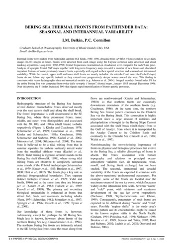
BELKIN AND CORNILLONlocated about 1 of latitude to the north of the front.The front thus appears to be related to the marginal icezone processes (Muench and Schumacher, 1985).Shallow fronts, tentatively identified as inner or uppershelf and coastal fronts, are observed off Alaskancoast, namely #10 off Kuskokwim Bay (persiststhrough November) and #11 in Shpanberg Strait andoff Norton Sound (disappears by October). Shallowfronts (##12-13) are observed off Anadyr Gulf; front#13 persists through November. Shelf-slope fronts##14-15 are associated with the Kamchatka Currentthat flows along the shelf break off Koryak Coast andoff Karaginsky and Olyutorsky bays. Front #16 hugsKomandorsky Islands. In June, shallow fronts persistoff Kuskokwim Bay, Norton Sound, and Anadyr Gulf(##4-6). The shelf-slope front (#2) is markedly nonisobathic. In July, the Norton Sound-Shpanberg StraitFront (#2) reaches south to Nunivak Island. Threeshallow fronts (##1, 6, and 7, or the coastal, uppershelf and inner shelf fronts, respectively) emerge inBristol Bay. In August, the entire Alaskan coast isrimmed by coastal and upper shelf fronts (##1, 2, 7,and 8). A seasonal shelf-slope (shelf break) front (#4)develops off Koryak Coast that persists throughNovember. In September, the Norton SoundShpanberg Strait Front (#2) begins its retreat to thenorth, whereas the Kuskokwim-Bristol Bays frontremains intact. The Bering Strait front (#3) connectsthe Bering Sea to the Chukchi Sea. In October, theinner shelf front (#1) appears along 50-m isobathwhile the mid-shelf front (#2) extends along 70-80misobath. Both fronts persist through November (##2and 3 respectively), when they are joined by a 30-misobath upper shelf front (#6) and shallow coastalfronts off Kuskokwim Bay (#8) and north of NunivakIsland (#9). Two fronts in the northwest correspond tothe northward Anadyr Current (#5) and southwardKamchatka Current (#4), both being branches of theBering Slope Current.Figure 2 shows all long-term monthly frontal pathscombined. It reveals the most persistent fronts, namely(from west to east), the Koryak, Anadyr, and BeringStrait fronts off Siberia’s coast; the Norton SoundShpanberg Strait front and Kuskokwim-Bristol baysfront off Alaska’s coast; the inner shelf front along the50-m isobath, and the mid-shelf front approximatelyalong the 70-80 m isobath. Other fronts are notablyless persistent, especially the shelf-slope (shelf break)front commonly believed to be associated with the 170m isobath. The main reason for the shelf-slope frontinstability is likely the very rugged bottom relief ofthe shelf break/continental slope areas. Indeed, thisarea is incised by a series of huge submarine canyons(Figure 1) that belong to the largest canyons in theWorld Oceans, namely Zhemchug Canyon (5,800km3, canyon volume), Navarin Canyon (5,400 km3),Pervenets Canyon (1,700 km3) and Pribilof Canyon(1,300 km3) that dwarf the largest NW Atlantic slopeincision, Hudson Canyon (300 km3) (Karl et al., 1996,Table 17-2).8 PAPERS PHYSICAL OCEANOGRAPHYSEASONAL AND INTERANNUALVARIABILITY OF FRONTAL ACTIVITYREVEALED BY INTEGRAL FRONTAL INDEXIn order to characterize spatially-integrated frontalactivity within our study area, the simplest possiblefrontal index has been calculated. This index, F1, is asum of frontal appearances within a study area. In ourcase, F1 is the total number of times each 9-km x 9km pixel contained an SST front. Since we focus onseasonal and interannual variability of fronts, dailyvalues of F1 were integrated over respective months.The resulting monthly index F1 reveals an extremelystrong seasonal variability that dominates interannualvariations over a 12-year study period, 1985-1996(Figure 10).To separate seasonal and interannual variability, thistime series has been time-averaged monthly andannually. Individual annual cycles (Figure 11) displaya strong year-to-year variability that modulates aunimodal seasonal cycle, which typically peaks inmid-summer. This seasonal pattern becomes apparentafter long-term monthly averaging (Figure 12).Long-term variability is revealed by annual averaging(Figure 13) that makes obvious an ascending trend ofF1, which increased approximately 50% from 1985through 1996.SUMMARYFive types of SST fronts have been provisionallyidentified over the Eastern Bering Shelf and Slope,loosely associated with certain depths or rather depthranges, namely (1) outer shelf front or shelf-slopefront (150 m and deeper); (2) mid-shelf front (70-80m); (3) inner shelf front (40-60 m); (4) upper shelffronts (25-35 m) and (5) coastal fronts (10-20m). TheNorton Sound-Shpanberg Strait front, Kuskokwimfront and Bristol Bay front are seasonally persistent.In the western Bering Sea, the Koryak-Kamchatkafront and especially Anadyr Gulf front are mostrobust. The entire frontal pattern changes notably onthe monthly scale. Most fronts are not strictlyisobathic. The inner shelf, upper shelf and coastalfronts are approximately isobathic, whereas the midshelf front and especially the shelf-slope (outer shelf)front do not follow any specific isobath as they extendover progressively deeper waters toward the west. Theintegral monthly frontal index F1 for the entire BeringSea exhibits an extremely strong seasonal variability,with a ten-fold increase from spring to summer and anabrupt drop in September. The annual mean monthlyfrontal index F1 increased approximately 50% from1985 through 1996, apparently signaling aconcomitant intensification of some yet unidentifiedfronto-genetic processes.PACIFIC OCEANOGRAPHY, Vol. 3, No. 1, 2005
BERING SEA THERMAL FRONTS FROM PATHFINDER DATA.Figure 1. Base map of the Bering Sea. Bottom relief is shown by three selected isobaths (blue lines), 50, 100and 200 m. Acronyms: BS, Bering Strait; NI, Nunivak Island; PI, Pribylof Island; SLI, St. Lawrence Island;SMI, St. Matthew Island;SS, Shpanberg Strait. Red polygon shows the frontal index F1 computation areaFigure 2. Seasonal variability of SST fronts, May-November, 1985-1996PACIFIC OCEANOGRAPHY, Vol. 3, No. 1, 2005PAPERS PHYSICAL OCEANOGRAPHY 9
BELKIN AND CORNILLONMAYFigure 3. SST fronts in May: long-term frequency (top), and frontal schematic (bottom)10 PAPERS PHYSICAL OCEANOGRAPHYPACIFIC OCEANOGRAPHY, Vol. 3, No. 1, 2005
BERING SEA THERMAL FRONTS FROM PATHFINDER DATA.JUNEFigure 4. SST fronts in June: long-term frequency (top), and frontal schematic (bottom)PACIFIC OCEANOGRAPHY, Vol. 3, No. 1, 2005PAPERS PHYSICAL OCEANOGRAPHY 11
BELKIN AND CORNILLONJULYFigure 5. SST fronts in July: long-term frequency (top), and frontal schematic (bottom)12 PAPERS PHYSICAL OCEANOGRAPHYPACIFIC OCEANOGRAPHY, Vol. 3, No. 1, 2005
BERING SEA THERMAL FRONTS FROM PATHFINDER DATA.AUGUSTFigure 6. SST fronts in August: long-term frequency (top), and frontal schematic (bottom)PACIFIC OCEANOGRAPHY, Vol. 3, No. 1, 2005PAPERS PHYSICAL OCEANOGRAPHY 13
BELKIN AND CORNILLONSEPTEMBERFigure 7. SST fronts in September: long-term frequency (top), and frontal schematic (bottom)14 PAPERS PHYSICAL OCEANOGRAPHYPACIFIC OCEANOGRAPHY, Vol. 3, No. 1, 2005
BERING SEA THERMAL FRONTS FROM PATHFINDER DATA.OCTOBERFigure 8. SST fronts in October: long-term frequency (top), and frontal schematic (bottom)PACIFIC OCEANOGRAPHY, Vol. 3, No. 1, 2005PAPERS PHYSICAL OCEANOGRAPHY 15
BELKIN AND CORNILLONNOVEMBERFigure 9. SST fronts in November: long-term frequency (top), and frontal schematic (bottom)16 PAPERS PHYSICAL OCEANOGRAPHYPACIFIC OCEANOGRAPHY, Vol. 3, No. 1, 2005
BERING SEA THERMAL FRONTS FROM PATHFINDER DATA.Figure 10. Temporal variability of the monthly frontal index F1Figure 11. Annual cycles of the monthly frontal index F1PACIFIC OCEANOGRAPHY, Vol. 3, No. 1, 2005PAPERS PHYSICAL OCEANOGRAPHY 17
BELKIN AND CORNILLONFigure 12. Mean seasonal cycle and its standard deviation (SD) of the monthly frontal index F1, 1985-1996Figure 13. Interannual variability of the mean monthly frontal index F118 PAPERS PHYSICAL OCEANOGRAPHYPACIFIC OCEANOGRAPHY, Vol. 3, No. 1, 2005
BERING SEA THERMAL FRONTS FROM PATHFINDER DATA.ACKNOWLEDGMENTSComments by Steve Okkonen and two anonymousreviewers helped us improve the manuscript. Thisstudy was funded by NASA through grants NAG53736 and NAG 512741 and by NOAA through theCooperative Institute for Arctic Research underNOAA Cooperative Agreement No. NA17RJ1224.The support of both agencies is greatly appreciated.REFERENCESAhlnäs K. and Garrison G.R. 1984. Satellite andoceanographic observations of the warm coastal current inthe Chukchi Sea, Arctic, 37(3), pp. 244-254.Belkin I.M. and Cornillon P.C. 2003. SST fronts of thePacific coastal and marginal seas, Pacific Oceanography,1(2), pp. 90-113.Belkin I.M. and Cornillon P.C. 2004. Surface thermalfronts of the Okhotsk Sea, Pacific Oceanography, 2(1-2),pp. 6-19.Belkin I.M., Cornillon P. and Ullman D. 2003. Ocean frontsaround Alaska from satellite SST data, Proceedings of theAmer. Met. Soc. 7th Conf. on the Polar Meteorology andOceanography, Hyannis, MA, Paper 12.7, 15 p.Benson A.J. and Trites A.W. 2002. Ecological effects ofregime shifts in the Bering Sea and eastern North PacificOcean, Fish and Fisheries, 3(2), pp. 95-113.Brodeur R.D., Wilson M.T. and Napp J.M. 1997.Distribution of juvenile pollock relative to frontal structurenear the Pribilof Islands, Bering Sea, in: Forage Fishes inMarine Ecosystems, Proc. Int'l Symp. on the Role of ForageFishes in Marine Ecosystems, Alaska Sea Grant CollegeProgram Rep. No. 97-01, University of Alaska Fairbanks.pp. 573-589.Brodeur, R.D., Mills C.E., Overland J.E., Walters G.E., andSchumacher J.D. 1999. Evidence for a substantial increasein gelatinous zooplankton in the Bering Sea, with possiblelink to climate change, Fish. Oceanogr., 8(4), pp. 296-306.Brodeur, R.D., Wilson M.T., and Ciannelli L. 2000. Spatialand temporal variability in feeding and condition of age-0walleye pollock (Theragra chalcogramma) in frontalregions of the Bering Sea, ICES J. Mar. Sci., 57(2), pp. 256264.Cayula J.-F., Cornillon P. 1992. Edge detection algorithmfor SST images. J. Atmos. Oceanic Tech., 9(1), pp. 67-80.Cayula J.-F., Cornillon P. 1995. Multi-image edgedetection for SST images. J. Atmos. Oceanic Tech., 12(4),pp. 821-829.Cayula J.-F., Cornillon, P. 1996. Cloud detection from asequence of SST images. Remote Sensing of Environment,55(1), pp. 80-88.Coachman L.K. 1986. Circulation, water masses, and fluxeson the southeastern Bering Sea shelf, Continental ShelfResearch, 5(1/2), pp. 23-108.Coachman L.K., Kinder T.H., Schumacher J.D., andTripp R.B. 1980. Frontal systems of the southeastern BeringSea shelf, in: Second International Symposium on StratifiedFlows, vol. 2, edited by T. Carstens and T. McClimans.Tapir, Trondheim. pp. 917-933,PACIFIC OCEANOGRAPHY, Vol. 3, No. 1, 2005Flint, M.V., Sukhanova I.N., Kopylov A.I., Poyarkov S.G.,and Whitledge T.E. 2002. Plankton distribution associatedwith frontal zones in the vicinity of the Pribilof Islands,Deep-Sea Res. II, 49(26), pp. 6069-6093.Gawarkiewicz G., Haney J.C. and Caruso M.J. 1994.Summertime synoptic variability of frontal systems in thenorthern Bering Sea, J. Geophys. Res., 99(C4), pp. 76177625.Gloersen P., Campbell W.J., Cavalieri D.J., Comiso J.C.,Parkinson C.L., and Zwally H.J. 1992. Arctic and AntarcticSea Ice, 1978-1987: Satellite Passive-MicrowaveObservations and Analysis. NASA SP-511, Washington,D.C., 290 p.Hansell D.A., Goering J.J., Walsh J.J., McRoy C.P.,Coachman L.K. and Whitledge T.E. 1989. Summerphytoplankton production and transport along the shelfbreak in the Bering Sea, Cont. Shelf Res., 9(12), pp. 10851104.Hunt G.L. and Stabeno P.J. 2002. Climate change and thecontrol of energy flow in the southeastern Bering Sea, Prog.Oceanogr., 55(1-2), pp. 5-22.Iverson R.L., Coachman L.K. Cooney R.T. English T.S.Goering J.J., Hunt G.L., Macauley Jr., M.C., McRoy C.P.,Reeburg W.S., Whitledge T.E., and Livingston R.J. 1979.Ecological significance of fronts in the southeastern BeringSea, in: Ecological Processes in Coastal and MarineSystems, Plenum Press, London. pp. 437-468.Johnson G.C., Stabeno P.J., and Riser S.C. 2004. TheBering Slope Current System Revisited, J. Phys. Oceanogr.,34(2), pp. 384-398.Kachel N.B., Hunt G.L. Jr., Salo S.A., Schumacher J.D.,Stabeno P.J., and Whitledge T.E. 2002. Characteristics andvariability of the inner front of the southeastern Bering Sea,Deep-Sea Res. II, 49(26), pp. 5889-5909.Karl H.A., Carlson P.R. and Gardner J.V. 1996. AleutianBasin of the Bering Sea: Styles of sedimentation and canyondevelopment, in: Geology of the United States’ seafloor:The view from GLORIA, ed. by J.V. Gardner, M.E. Field,and D.C. Twichell, Cambridge University Press, New York,pp. 305-332.Kinder T.H. and Coachman L.K. 1978. The frontoverlaying the continental slope in the eastern Bering Sea, J.Geophys. Res., 83(C9), pp. 4551-4559.Kinder T.H. and Schumacher J.D. 1981a. Hydrographicstructure over the continental shelf of the southeasternBering Sea, in: The Eastern Bering Sea Shelf:Oceanography and Resources, Volume 1, edited by D.W.Hood and J.A. Calder, NOAA, University of WashingtonPress, Seattle. pp. 31-52.Kinder T.H. and Schumacher J.D. 1981b. Circulation overthe continental shelf of the southeastern Bering Sea, in: TheEastern Bering Sea Shelf: Oceanography and Resources,PAPERS PHYSICAL OCEANOGRAPHY 19
BELKIN AND CORNILLONVolume 1, edited by D.W. Hood and J.A. Calder, NOAA,University of Washington Press, Seattle. pp. 53-75.Kinder T.H.,Hunt G.L.Jr.,Schneider D.,andSchumacher J.D. 1983. Correlations between seabirds andoceanic fronts around the Pribilof Islands, Alaska,Estuarine, Coastal and Shelf Science, 16(3), pp. 303-319.Kowalik Z. 1999. Bering Sea tides, in: Dynamics of theBering Sea, edited by T.R. Loughlin and K. Ohtani,University of Alaska Sea Grant, AK-SG-99-03, Fairbanks.pp. 93-127.Luchin V.A., Semiletov I.P. and Weller G.E. 2002. Changesin the Bering Sea region: atmosphere-ice-water system inthe second half of the twentieth century, Prog. Oceanogr.,55(1-2), pp. 23-44.Lynch A.H., Glueck M.F., Chapman W.L., Bailey D.A., andWalsh J.E. 1997. Satellite observation and climate systemmodel simulation of the St. Lawrence Island polynya,Tellus, 49A(2), pp. 277-297.Maynard N.G., and Clark D.K. 1987. Satellite colorobservations of spring blooming in Bering Sea shelf watersduring the ice edge retreat in 1980, J. Geophys. Res.,92(C7), pp. 7127-7139.Muench R.D., and Schumacher J.D. 1985. On the BeringSea ice edge front, J. Geophys. Res., 90(C2), pp. 3185-3197.NASA. 1998. Sea ice concentrations from Nimbus-7 SMMRand DMSP SSM/I passive microwave data, 1978-1996,Volumes 1-3 (on CD-ROMs; USA NASA 971 0001,0002, 0003), Goddard Space Flight Center, Laboratory forHydrospheric Processes. Archived and distributed byNSIDC, CIRES, University of Colorado Boulder.Nasu K. 1974. Movement of baleen whales in relation tohydrographic conditions in the northern part of the NorthPacific Ocean and the Bering Sea, in: Oceanography of theBering Sea with emphasis on renewable resources, edited byD.W. Hood and E.J. Kelley, Institute of Marine Science,University of Alaska, Fairbanks. pp. 345-361.Niebauer H.J. 1998. Variability in Bering Sea ice cover asaffected by a regime shift in the North Pacific in the period1947-1996, J. Geophys. Res., 103(C12), pp. 27717-27737.Okkonen S.R., Schmidt G.M., Cokelet E.D. and StabenoP.J. 2004. Satellite and hydrographic observations of theBering Sea 'Green Belt', Deep Sea Res. Part II: TopicalStudies in Oceanography, 51(10-11), pp. 1033-1051.Overland J.E., and Stabeno P.J. 2004. Is the climate of theBering Sea warming and affecting the ecosystem, Eos,85(33), pp. 309-312.Polovina J.J., Mitchum G.T., Graham N.E., Craig M.P.,Demartini E.E., and Flint E.N. 1994. Physical and biologicalconsequences of a climate event in the central North Pacific,Fisheries Oceanography, 3(1), pp. 15-21.Russell R.W., Harrison N.M., and Hunt G.L., Jr. 1999.Foraging at a front: Hydrography, zooplankton, and avianplanktivory in the northern Bering Sea, Mar. Ecol. Prog.Ser., 182, pp. 77-93.20 PAPERS PHYSICAL OCEANOGRAPHYSaitoh S.-I., Eslinger D., Sasaki H., Shiga N., Odate T., andMiyoi T. 1998. Satellite and ship observations of coastalupwelling in the St. Lawrence Island Polynya (SLIP) area insummer, 1994 and 1995, Mem. Fac. Fish. Hokkaido Univ.,45(1), pp. 18-23.Schneider D. 1982. Fronts and seabird aggregations in thesoutheast Bering Sea, Mar. Ecol. Prog. Ser., 10(1), 101-103.Schneider D., Harrison N.M., and Hunt G.L., Jr. 1987.Variation in the occurrence of marine birds at fronts in theBering Sea, Estuarine, Coastal and Shelf Science, 25(1),pp. 135-141.Schumacher J.D., Kinder T.H., Pashinski D.J., andCharnell R.L. 1979. A structural front over the continentalshelf of the eastern Bering Sea, J. Phys. Oceanogr., 9(1),pp. 79-87.Schumacher J.D., and Stabeno P.J. 1998. Continental shelfof the Bering Sea, in: The Sea, vol. 11, edited by A.R.Robinson and K.H. Brink, John Wiley and Sons, New York.pp. 789-822.Springer A.M., McRoy C.P., and Flint M.V. 1996. TheBering Sea Green Belt: shelf-edge processes and ecosystemproduction, Fish. Oceanogr., 5(3/4), pp. 205-223.Stabeno P.J., Schumacher J.D. and Ohtani K. 1999a.Physical oceanography of the Bering Sea, in: Dynamics ofthe Bering Sea, edited by T.R. Loughlin and K. Ohtani,University of Alaska Sea Grant, AK-SG-99-03, Fairbanks.pp. 1-26.Stabeno P.J., Schumacher J.D., Salo S.A., Hunt G.L. Jr. andFlint M. 1999b. Physical environment around the PribilofIslands, in: Dynamics of the Bering Sea, edited by T.R.Loughlin and K. Ohtani, University of Alaska Sea Grant,AK-SG-99-03, Fairbanks. pp. 193-215.Stabeno P.J., Bond N.A., Kachel N.B., Salo S.A., andSchumacher J.D. 2001. On the temporal variability of thephysical environment over the south-eastern Bering Sea,Fish. Oceanogr., 10(1), pp. 81-98.Tynan C.T., DeMaster D.P., and Peterson W.T. 2001.Endangered right whales on the southeastern Bering Seashelf, Science, 294(5548), 1894.Verkhunov A.V. 1994. Thermohaline characteristics ofshelf fronts in the western Bering Sea, Oceanology, Englishtranslation, 34(3), pp. 321-333.Vidal J., and Smith S.L. 1986. Biomass, growth anddevelopment of populations of herbivorous zooplankton inthe southeastern Bering Sea during spring, Deep-Sea Res.,33(4), pp. 523-556.Walsh J.E., Dieterle D.A., Muller-Karger F.E., Aagaard K.,Roach A.T., Whitledge T.E., and Stockwell D. 1997. CO2cycling in the coastal ocean. II. Seasonal organic loading ofthe Arctic Ocean from source waters in the Bering Sea,Cont. Shelf. Res., 17(1), pp. 1-36.Wyllie-Echeverria T., and Ohtani K. 1999. Seasonal seaice variability and the Bering Sea ecosystem, in: Dynamicsof the Bering Sea, edited by T.R. Loughlin and K. Ohtani,University of Alaska Sea Grant, AK-SG-99-03, Fairbanks.pp. 435-451.PACIFIC OCEANOGRAPHY, Vol. 3, No. 1, 2005
Graduate School of Oceanography, University of Rhode Island (URI), USA Email: ibelkin@gso.uri.edu Thermal fronts were studied from Pathfinder satellite SST fields, 1985-1996, obtained from AVHRR 9-km resolution twice-daily images (8,364 images in total). Fronts were detected from each image using the Cayula-Cornillon edge detection and cloud